How to compute index numbers at top speed

In several data models, you need to assign an index number to a row. The index is an incremental number that sorts the rows according to some rule. For example, you might want to assign an index to sales, so to be able to find the first or the second of a given customer. In this article, we analyze a naïve approach, which turns to be very slow, and an optimized one, using the RANKX function.

Imagine that – given a customer – you want to assign an index number to its sale events, in order to identify all the sales of a customer, finding the first transaction, the second one, and so on. This might be useful to compute the purchase frequency of a customer and categorize him based on that information.

The simplest way of computing such a number is through a calculated column that looks like this:

Sales[CustomerSaleIndex] = 
VAR CurrentOrderDate = Sales[Order Date]
VAR CurrentCustomerKey = Sales[CustomerKey]
RETURN
COUNTROWS ( 
    FILTER ( 
        Sales,
        AND ( 
            Sales[Order Date] < CurrentOrderDate,
            Sales[CustomerKey] = CurrentCustomerKey
        )
    )
) + 1

The code is pretty simple, and – to be honest – we have shown code similar to this in many articles and books, because it looks like a simple and intuitive way of computing an index. Unfortunately, the major drawback of this code is that it takes forever to run even on relatively small tables. In fact, we tried this code on the Contoso database that we normally use for demos, where the Sales table contains 12 millions of rows. After 15 minutes, the calculated column was not there yet, exhausting in this way not only our patience, but also the memory of the laptop used for the tests (16GB). In other words, memory filled up and we did not get any answer, apart an out-of-memory error. It is not that the code does not work, it will eventually return a correct result on a larger server, but performance and memory usage are definitely big problems here.

Luckily, there is a good alternative way of obtaining the same result, which is leveraging the RANKX function. RANKX is designed (and optimized) to provide the ranking of an expression over a lookup table. What if we use RANKX to provide the ranking of the current sale against all the sales of the current customer? The algorithm is the same, the only difference is that – now – we leverage a built-in function to obtain the same result, hoping that the SSAS team spent time optimizing RANKX in a better way.

Thus, we tried this different formulation of the same calculation:

Sales[CustomerSaleIndex] = 
VAR CurrentCustomerKey = Sales[CustomerKey]
RETURN
RANKX ( 
    FILTER ( 
        Sales, 
        Sales[CustomerKey] = CurrentCustomerKey 
    ), 
    Sales[Order Date], , ASC, Dense
)

Surprisingly, the calculated column is computed and saved in a couple of seconds. Definitely a much better pattern, if you need to compute index numbers. If you look at the demo file, please note that the two index might return different values in the presence of ties, this is expected (and, by the way, we strongly prefer the RANKX version)

This – of course – raised our curiosity to better understand the differences between the two functions. Since monitoring the execution plan of a calculated column is not an easy task, we decided to try with a query, which is easier to follow. Of course, we did not want to perform the analysis on the Sales table, which would lead to a huge execution time, so we tried the same pattern on the customer table, which is a much better candidate because it contains only 18.000 rows.
This is the query we executed to test the first approach:

EVALUATE
ADDCOLUMNS (
    ALL ( Customer[Customer Code] ),
    "Index", COUNTROWS (
        FILTER (
            Customer,
            Customer[Customer Code] 
                <= EARLIER ( Customer[Customer Code] )
        )
    )
)

Being a smaller table, it did not eat all memory and it returned the result in 1 minute and 37 seconds, which means forever in DAX terms. The optimized version of the same query is the following one:

EVALUATE
ADDCOLUMNS (
    ALL ( Customer[Customer Code] ),
    "Index", RANKX ( Customer, Customer[Customer Code] )
)

This latter version runs in 89 milliseconds. Thus, the ratio between the two is 97,589 / 89, more than 1,000 times faster. We then tested the same pattern in different scenarios, and we consistently found that RANKX is amazingly fast when compared to the more common pattern of using COUNTROWS with FILTER.

A deeper analysis at the query plan shows that the first query, with the FILTER call, needs to iterate all the customer codes and, for each one, it scans the customer codes again in order to compute the list of all the rows that happen to be less than the current one.

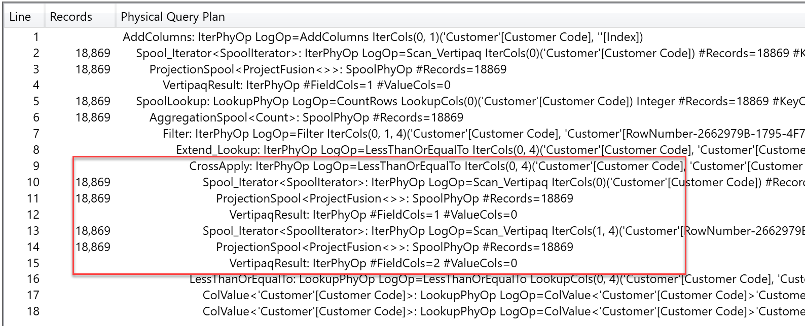
This is exactly what the query is asking for, so we are not surprised by that. What is surprising is the fact that the RANKX query plan shows a different pattern.

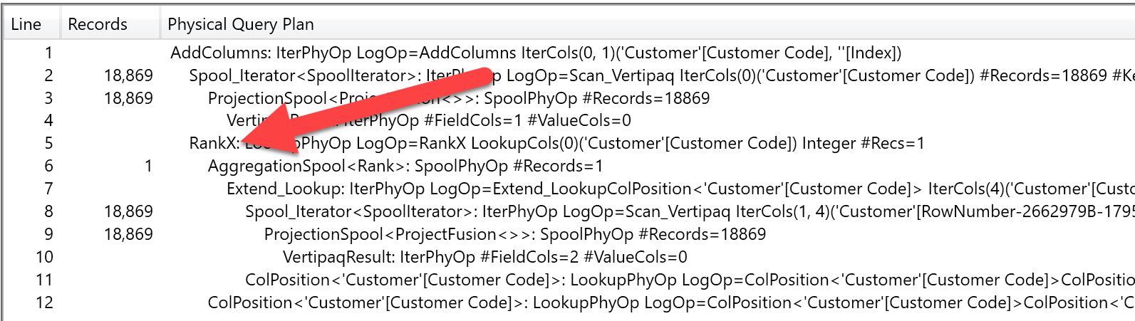
It still iterates over 18,000 rows but, for each one, it executes a single call to the RankX operator, which works on the list of codes and computes the ranking. Clearly, the RankX physical engine operator is very well optimized, so it does not need to iterate and sort the whole list every time it is called.

The query optimizer can understand the RANKX pattern very well, even if the code is more complex. For example, a different – and more complex – index number is the ranking of a customer based on sales in its continent. You can write the code with RANKX in this way:

EVALUATE
ADDCOLUMNS (
    ALL ( Customer ),
    "Index",
    VAR CurrentContinent = Customer[Continent]
    RETURN
        RANKX (
            FILTER ( 
                Customer, 
                Customer[Continent] = CurrentContinent 
            ),
            CALCULATE ( SUM ( Sales[Quantity] ) )
        )
)

Or, if you want to write it without RANKX, then you need a slightly more complex piece of DAX:

EVALUATE
ADDCOLUMNS (
    ALL ( Customer ),
    "Index",
    VAR CurrentContinent = Customer[Continent]
    VAR CurrentSalesQuantity = CALCULATE ( SUM ( Sales[Quantity] ) )
    RETURN
        COUNTROWS (
            FILTER (
                Customer,
                AND (
                    Customer[Continent] = CurrentContinent,
                    CALCULATE ( SUM ( Sales[Quantity] ) ) 
                        >= CurrentSalesQuantity
                )
            )
        )
)

The RANKX version runs in less than one second, whereas the non-RANKX one runs in more than 22 seconds. The query plan, although much more complex, shows a similar pattern: Using RANKX, the engine does not need to iterate over the CROSSJOIN of customers, but it uses the optimized RankX operator.

If you need index numbers computed in your model, try to compute them using RANKX instead of COUNTROWS, it is likely that the performance of your model will have a great benefit.