 Alberto Ferrari
Auto-exist is the feature of SSAS that shows, in the result of queries, only existing combinations of attributes. If, for example, you do not sell any blue shirt, you would not expect the combination of blue and shirt to appear in any of your PivotTables, even if you sell blue bikes and white shirts. Color and product category are on different columns, but auto-exist takes care of this, ensuring that the result of a query contains only existing combinations of attributes.
We will show one of the scenarios where auto-exist behavior might surprise you, and we will take this as an opportunity to dig a bit deeper in the understanding of evaluation contexts. As an example, consider the canonical AdventureWorks data model, with products, categories and subcategories.
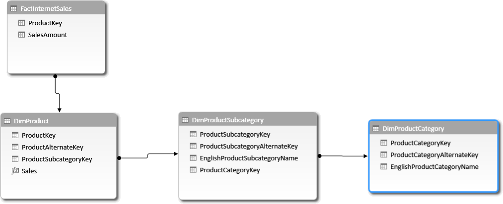
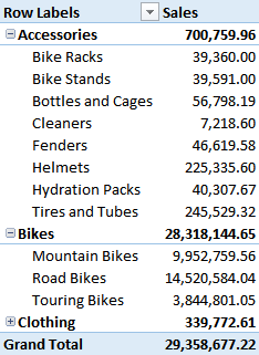
Based on this model, you can easily build a PivotTable that shows category, subcategory and sales. You will see only existing combinations of category and subcategory:
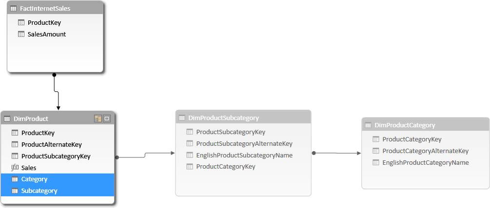
You can modify the data model, denormalizing the category and subcategory names in the DimProduct table, to make it easier to browse. To improve usability, you hide the two related dimensions:
If you build a similar PivotTable, you will get the very same result, i.e. only existing combinations of category and subcategory will show up in the PivotTable. For example, the pair Accessories and Road Bikes will not appear, because such a combination does not exist in the data.
Thus, it looks like the two models are the very same, right? Wrong. Even if the two PivotTables show the very same result, their internal behavior is different. This might lead to some unexpected results. In order to understand what is happening, you can put the PivotTable side by side and then enable, on both, the display of items with no data, using the PivotTable options:
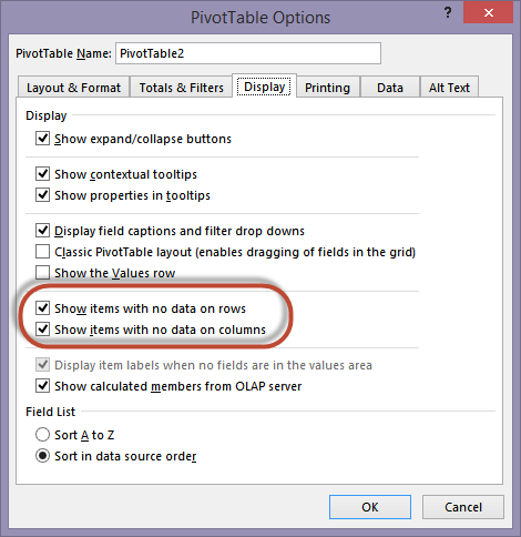
Once you have done this, the two PivotTable will show different results:
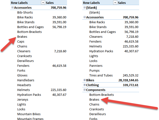
In the left PivotTable, I used the normalized category and subcategory, i.e. the values from the DimProductCategory and DimProductSubcategory tables. In the right one, I used category and subcategory in the DimProduct table. You can see that the pair (Accessories, Brakes), which does not exist in the database, is shown in the left PivotTable and hidden in the right one. Brakes is a subcategory of Components, not of Accessories. In fact, in the right PivotTable, it appears under the Components list of subcategories.
Why is this happening? Because two different mechanisms are working, leading to a similar result, but in different ways: auto-exist and empty-rows removal. Auto-exists is a feature working at the server level. Auto-exists makes non-existing combinations of attributes invisible to any client tool that queries your database. Empty-rows removal is a PivotTable feature that hides rows containing only blank values in the measures.
When you disable empty-rows removal, both PivotTables show rows containing only blank values, but the left one is showing non-existing combinations, whereas the right one shows only existing combinations. Because we disabled empty-rows removal, there should be something different in the behavior of auto-exist.
Auto-exist works only among columns in the same table, by default. Said in other words, if you project on a PivotTable two columns of the same table, then auto-exist will make sure that only existing combinations of the two columns will be returned as part of the result. If, on the other hand, the two columns are coming from different tables, then auto-exist does no longer activate and the engine will evaluate and return all of the combinations, possibly with blank results. The PivotTable hides blank results and makes the two sets appear identical even if, internally, they resulted in a very different calculation.
You might wonder, at this point, why you should worry about internal aspects like this one. At the end, the result is the same and the user will never notice any difference when browsing the model. In reality, ignoring this aspect might lead to unexpected results, which might confuse even seasoned developers.
Imagine you define a measure like the following one in the denormalized model:
SalesOfBikes :=
CALCULATE (
    [Sales],
    DimProduct[Category] = "Bikes"
)
If you put it in the PivotTable, you will see this result:
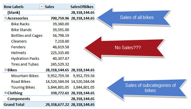
Because the CALCULATE function replaces the filter on the DimProduct[Category] column, you will get:
- Total sales of bikes, when Category is already filtered, because the filter is replaced.
- No sales, when both Category and Subcategory are filtered, because the filter on Category is replaced and the filter on Subcategory is still active. This is the most surprising result, but it makes sense after you think for a minute about it.
- Sales of the subcategory of Bikes, when the filter on Category is the same as the one being replaced.
If, on the other hand, you write the same calculation, albeit somewhat different, on the normalized model, you will write this code:
SalesOfRelatedBikes :=
CALCULATE (
    [Sales],
    DimProductCategory[EnglishProductCategoryName] = "Bikes"
)
A PivotTable with DimProductCategory and DimProductSubcategory to slice the values shows a completely different result between Sales and SalesOfRelatedBikes measures:
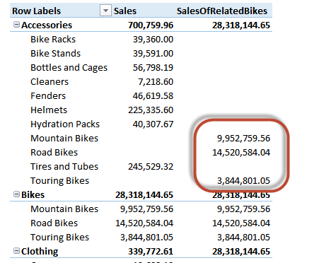
You can see that the boxed numbers refer to non-existing combinations of category and subcategory. In fact, the combination (Accessories, Road Bikes) does not exist in the database. Yet, you see the sales of road bikes as part of the Accessories category. This combination, of course, was not visible in the previous model.
Because the two column used in the PivotTable belong to different tables, auto-exist is not active. Thus, all of the combinations of the two columns are evaluated, even the ones which would normally lead to a blank result. However, because in the formula you override the filter on EnglishCategoryName, the combination (Accessories, Road Bikes) becomes (Bikes, Road Bikes) and this combination has a value, i.e. the sales of road bikes. The PivotTable then shows the value under the (Accessories, Road Bikes) cell, which seems to make no sense.
In reality, the behavior is correct, if you think in terms of auto-exist logic. Nevertheless, you might be surprised by the result, if you do not think that the two mechanism (blank removal and auto-exist) are different.
There are, of course, many ways to write a DAX measure in a normalized model that mimic auto-exist, and we suggest you to find them, so to get a better understanding of how auto-exist works in a model. One example might be:
SalesOfBikes :=
CALCULATE (
    [Sales],
    DimProductCategory[EnglishProductCategoryName] = "Bikes",
    CALCULATETABLE (
        DimProductCategory,
        FILTER (
            ALL ( DimProductSubcategory ),
            IF (
                ISFILTERED ( DimProductSubcategory[EnglishProductSubcategoryName] ),
                CONTAINS (
                    VALUES ( DimProductSubcategory ),
                    DimProductSubcategory[ProductSubcategoryKey], DimProductSubcategory[ProductSubcategoryKey]
                ),
                TRUE
            )
        )
    )
)
The goal of this article is not that of solving a specific problem, but pointing your attention on a behavior of tabular data models that might surprise you, if you have never seen it before.
Evaluates an expression in a context modified by filters.
CALCULATE ( <Expression> [, <Filter> [, <Filter> [, … ] ] ] )