 Marco Russo & Alberto Ferrari
At the core of any business intelligence solution lies its data model. Power BI is no exception: a quality data model lets you build solid and powerful solutions that will work like a breeze for many years. A poor data model might oftentimes be the reason the entire project fails. The speed, reliability, and power of a solution all stem from the same origin: a good data model. We dare add: if the project is doomed to fail, better for it to fail as soon as possible. A project developed for years and based on the wrong model will fall from a greater height and only cause more damage.
The data model is the first choice you have to make as a BI developer, and you want to choose right. Because of the importance of the data model, over the past few years BI developers have spent a lot of energy towards designing patterns and techniques that guarantee solid foundations for a project. The fruit of this huge undertaking was the definition of star schemas. If you ask a seasoned BI developer how to build a correct data model, you will always obtain the same answer: build a star schema. At SQLBI, we are no exception. Star schemas are at the core of the data modeling training courses that we have designed and that we deliver.
The reason experienced BI professionals always choose a star schema is because they have failed several times with other models. All those times, the solution to their problems was to build a star schema. You may make one, two, ten errors. After those, you learn to trust star schemas. This is how you become an expert: after tons of errors, you finally learn how to avoid them.
Sometimes, the person in charge of making such an important decision has not failed enough times, and they give in to the temptation of trying a different model. Among the many different inclinations they may have, one is really tempting: the single, large table. The internal monologue typically goes something like this:
Why should I have products, sales, date and customers as separate tables? Wouldn’t it be better to store everything in a single table named Sales that contains all the information? After all, every query I will ever run will always start from Sales. By storing everything in a single table, I avoid paying the price of relationships at query time, therefore my model will be faster.
There are multiple reasons why a single, large table is not better than a star schema. Here anyway, the focus is strictly on performance. Is it true that a single table is faster than a star schema? After all, we all know that joining two tables is an expensive operation. So it seems reasonable to think that removing the problem of joins ends up in the model being faster. Besides, with the advent of NOSQL and big data, there are so many so-called data lakes holding information within one single table… Isn’t it tempting to use those data sources without any transformation?
I wanted to provide a rational answer to the question – an answer based solely on numbers.
Beware: the remaining part of the article goes into quite a high level of technical detail. If you want to just read the conclusions, you can jump to the end of the article. However, there is value in looking at the numbers if you want to better follow my reasoning.
The test setup
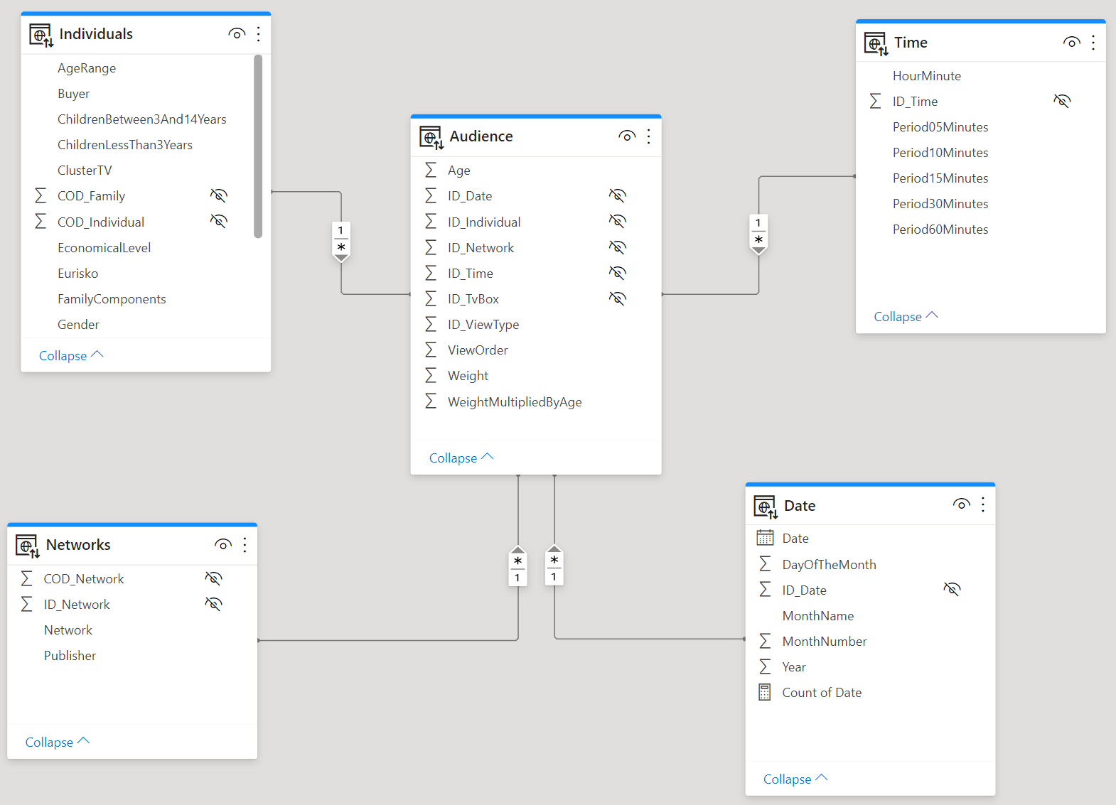
We built two models. One is using a regular star schema, with four dimensions around a single fact table.
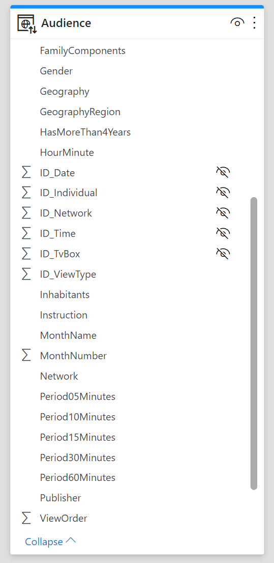
The other model contains the same information, but the dimensions are gone. All the columns from the dimensions have been denormalized into the fact table.
Because the denormalized model is based on a “big fat table”, we call the models “fat” and “slim”. Moreover, in order to make the differences between the different measurements visible, we used a rather large model as the main fact table contains 4 billions rows. This way, the time required to scan the table is large enough to make it easy to spot the differences between the two models.
All the tests are being executed on a powerful machine. It uses an AMD Ryzen Threadripper 3970X with 32 physical cores and 64 virtual cores. The size of the table and the number of cores means that the degree of parallelism obtained by the storage engine is huge. For this reason, we are mainly interested in the storage engine CPU values, to obtain a clear picture of the amount of CPU power required to answer the queries. Indeed, there might be no visible differences between a query that runs in 100 milliseconds or in 10 milliseconds. However, when you multiply that number by the number of cores used, the difference definitely becomes relevant! The storage engine (SE) CPU value measures the total CPU power required to run the query, and it is the main metric we use in the article. We used an on-premises instance of Analysis Services 2019 to perform all the tests.
Database size
The first important difference between the two models is their size. The slim model uses 16.80 GB of RAM, whereas the fat model uses 44.51 GB of RAM. The fat model is 2.65 times the size of the slim model. Both models were processed with the default configuration of Analysis Services.
Why are the models so different in size? Because there are a huge number of columns in the fat model! In the slim model, the largest column is the time key (ID_Time). The column is so large because there is a value for each second in time.
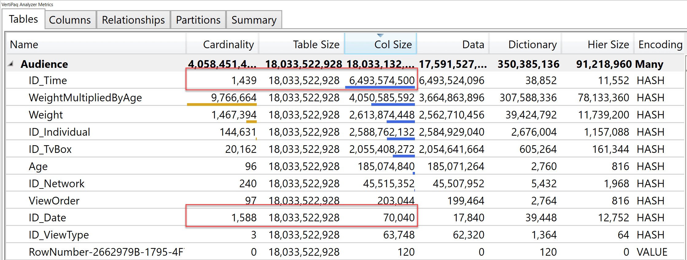
If you compare ID_Time with ID_Date you have a better picture: despite having the same cardinality, date changes very slowly compared with time. Therefore, the run-length encoding (RLE) algorithm of VertiPaq obtains a much better compression for date than it ever could with time. This is a characteristic of VertiPaq: columns that change frequently result in being larger, therefore slower.
In the star schema, ID_Time is the key that ties the fact table with the Time dimension. In the fat model, there is no time dimension: all the columns of Time have been denormalized in the fact table. Therefore, each of those columns has a very large size, depending on how frequently the values inside change.
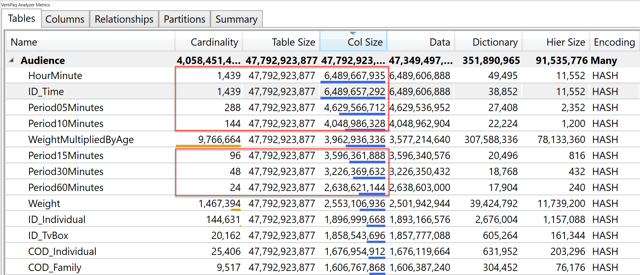
Despite it being larger, we expect the fat model to perform better on certain queries. Indeed, imagine a query that needs to group by Period05Minutes and produce the sum of a column. In the slim model VertiPaq needs to traverse a relationship that uses the ID_Time column. It must scan 6.5 GB of data. The same query on the fat model scans the Period05Minutes column in the fact table, which is only 4.6 GB. The difference is not only due to the presence of the relationship, but more importantly to the size of the columns involved in the query. The benefit of the fat model depends on how large the columns used for the aggregation are.
Now that we have taken a look at the model, we start running queries of different complexity and measure their speed on the two models.
Simple sum, grouping by small column
The first query groups by the AgeRange column, which is an attribute of Individuals. AgeRange contains only 96 distinct values, but it belongs to a dimension with 144K rows. When denormalized in the fat model, the AgeRange column uses only 42 MB of data. The key of the relationship, on the other hand, uses 2.5 GB. Therefore, the slim model deals with the time required to traverse the relationship, but also with the increase in size of the columns involved:
EVALUATE
SUMMARIZECOLUMNS (
    Individuals[AgeRange],
    "Weight", SUM ( Audience[Weight] )
)
Below, you find the server timings on the slim model.
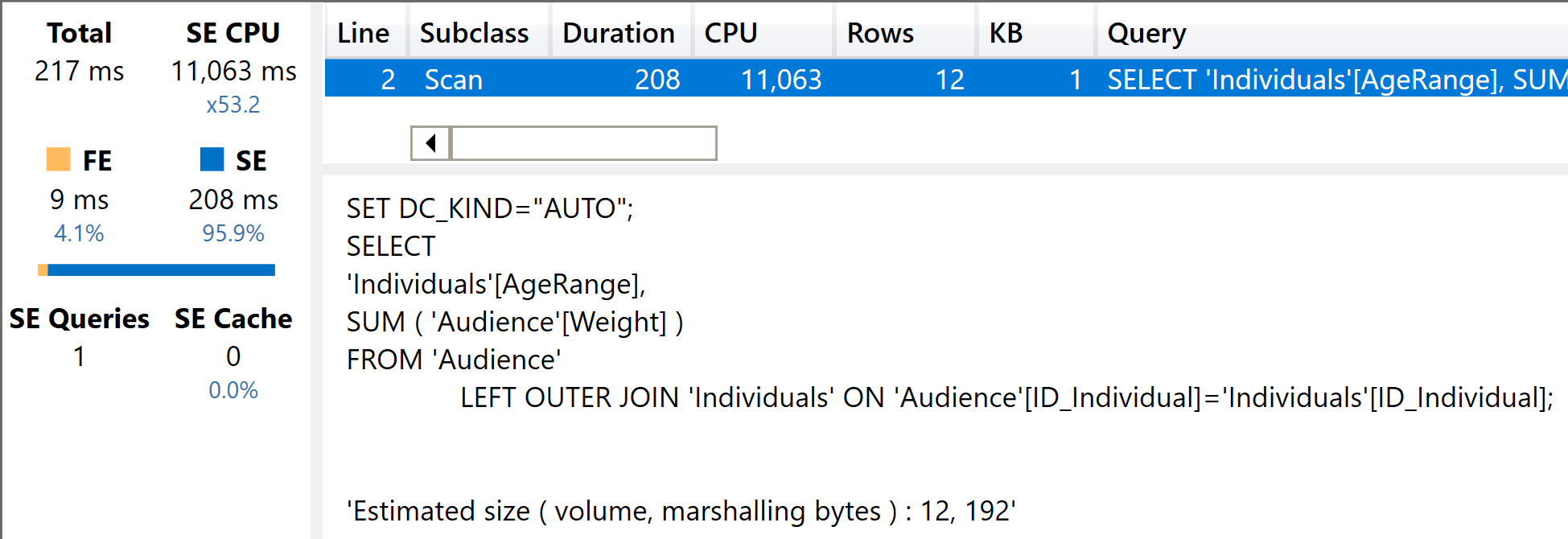
The query used around 11 seconds of CPU, and you can clearly see the JOIN executed by the storage engine. The same query executed on the fat model is much faster. Here is the query:
EVALUATE
SUMMARIZECOLUMNS (
    Audience[AgeRange],
    "Weight", SUM ( Audience[Weight] )
)
And below is the result of the execution.
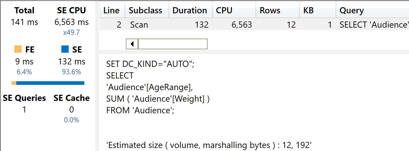
Six and a half seconds, compared to eleven seconds in the slim model. As expected, the fat model is much faster for this specific query.
Simple sum, grouping by large column
The second test is similar to the first, only this time we use the Period05Minutes column that is much larger than AgeRange. The fat model is still faster; that said, the size of the column now starts to weigh in thus largely reducing the benefit of the fat model.
Here is the second query on the slim model:
EVALUATE
SUMMARIZECOLUMNS (
    Time[Period05Minutes],
    "Weight", SUM ( Audience[Weight] )
)
The execution time is larger than before, because of the size of the relationship.
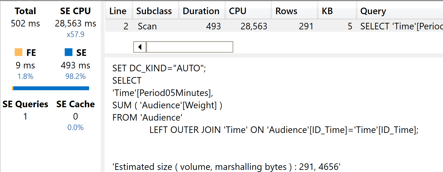
As was the case earlier, you see that there is a single JOIN with the dimension used in the query. The query runs with a great degree of parallelism: the total execution time is just half a second and yet the total SE CPU time went up to 28 seconds.
The query on the fat model is identical, except for the table used:
EVALUATE
SUMMARIZECOLUMNS (
    Audience[Period05Minutes],
    "Weight", SUM ( Audience[Weight] )
)
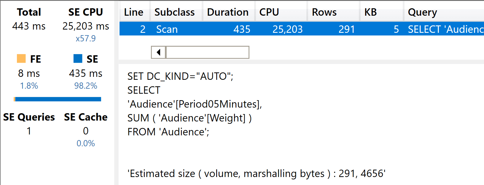
On the fat model, the performance is still better, even if some of the advantage that was present with the smaller column is lost.
Both results so far are as expected. The fat model is faster. The important detail here is, “how much faster?” If you focus only on the first query, it seems to run twice as fast. But in reality, as soon as the query becomes more complex or the columns used increase in size, the difference becomes smaller.
Simple sum, grouping by multiple columns
The first two tests used only one column to perform the grouping. What if we increased the number of columns? I was expecting the benefit of the fat model to lessen, due to the larger size of the columns involved. Instead, quite surpringly the ratio remained almost the same between the two models.
Here is the query on the slim model. It is using three columns from the same dimension:
EVALUATE
SUMMARIZECOLUMNS (
    Time[Period60Minutes],
    Time[Period10Minutes],
    Time[Period05Minutes],
    "Weight", SUM ( Audience[Weight] )
)
And here you see the result of the execution.
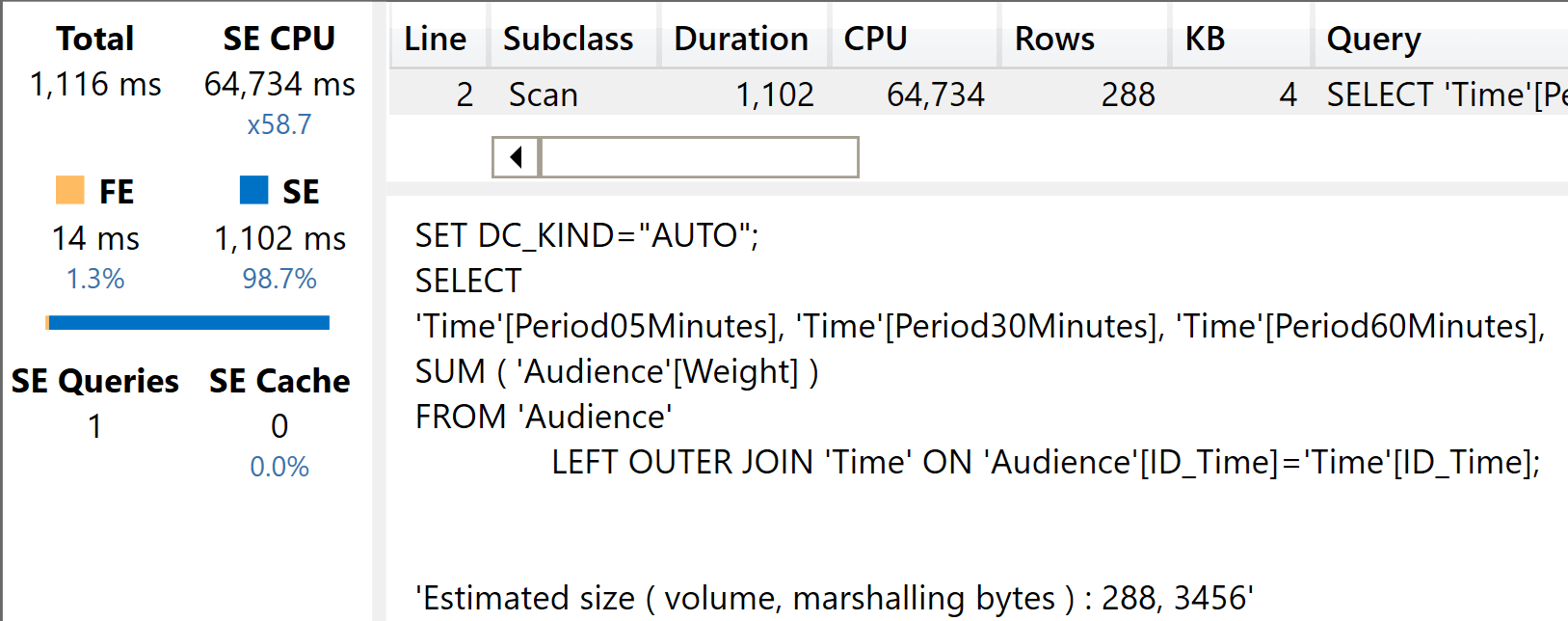
It took 64 seconds of CPU time, more than double the time required to group by only one column. This is quite surprising because the cardinality of the scan is the same as the cardinality of the previous query, that was using only the Period05Minutes column. Indeed, the highest detail is still 5 minutes: we only added two additional columns to the result.
In the fat model, the only change is the table name of the columns used in the groupby part:
EVALUATE
SUMMARIZECOLUMNS (
    Audience[Period60Minutes],
     Audience [Period10Minutes],
     Audience [Period05Minutes],
    "Weight", SUM ( Audience[Weight] )
)
The result on the fat model is not very different from the previous test.
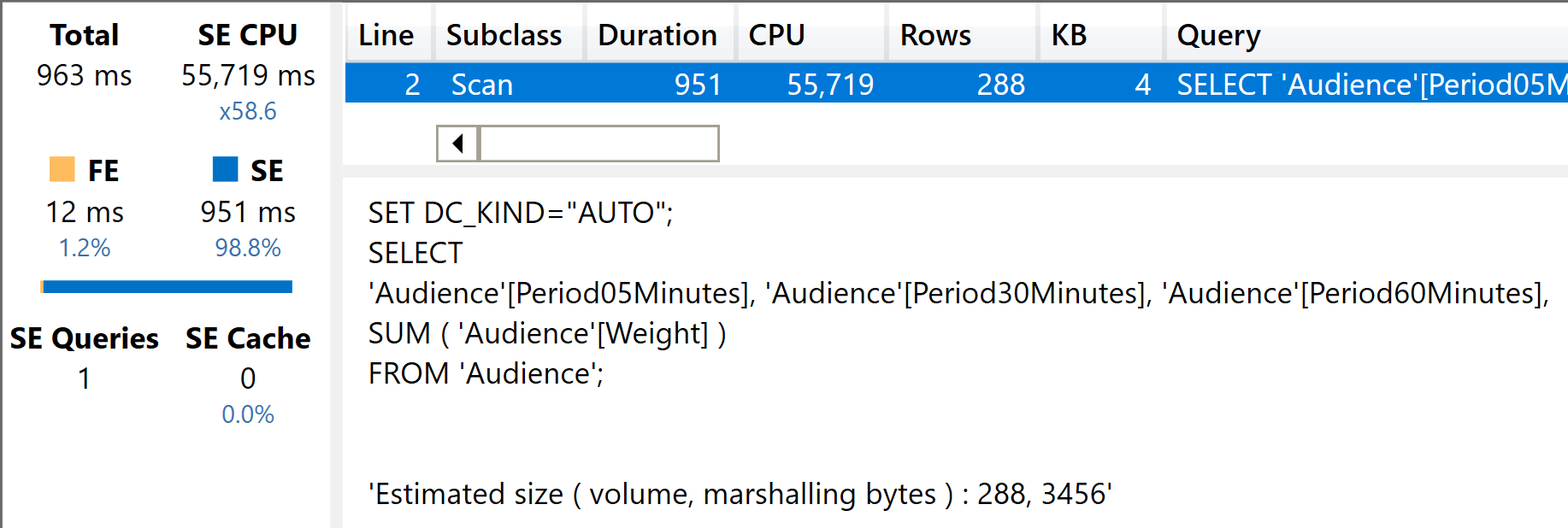
This result is not unexpected: because the number of large columns is higher, it is totally expected for the query to be slower than the one with a single column. In percentage, it maintained its advantage against the slim model.
I have to say that this result surprised me. I would have expected the slim model to perform much better. Now, I know I need to investigate more on the behavior of VertiPaq with multiple columns in a star schema. I will update the article (or publish a new one) as soon as I understand why the slim model performed so poorly.
Distinct count on slowly-changing dimensions
So far, we have been computing values by using a simple SUM. An interesting question is whether we can keep the same difference with a heavier calculation, like a distinctcount. There are two interesting columns to use for a distinct count: the person key (ID_Individual) and the person code (COD_Individual). Because Individual is a slowly-changing dimension, we can expect a significant difference between the two models. Indeed, with the fat model both distinct counts can be executed by scanning one table, whereas the slim model requires a join when computing the distinct count of COD_Individual. This is because this column is stored in Individuals, not in the fact table.
Let us start with the surrogate key, where both the fat and slim model need to query only the fact table:
EVALUATE
SUMMARIZECOLUMNS(
    Time[Period05Minutes],
    "Test", DISTINCTCOUNT ( Audience[ID_Individual] )
)
Here is the distinct count on the slim model.
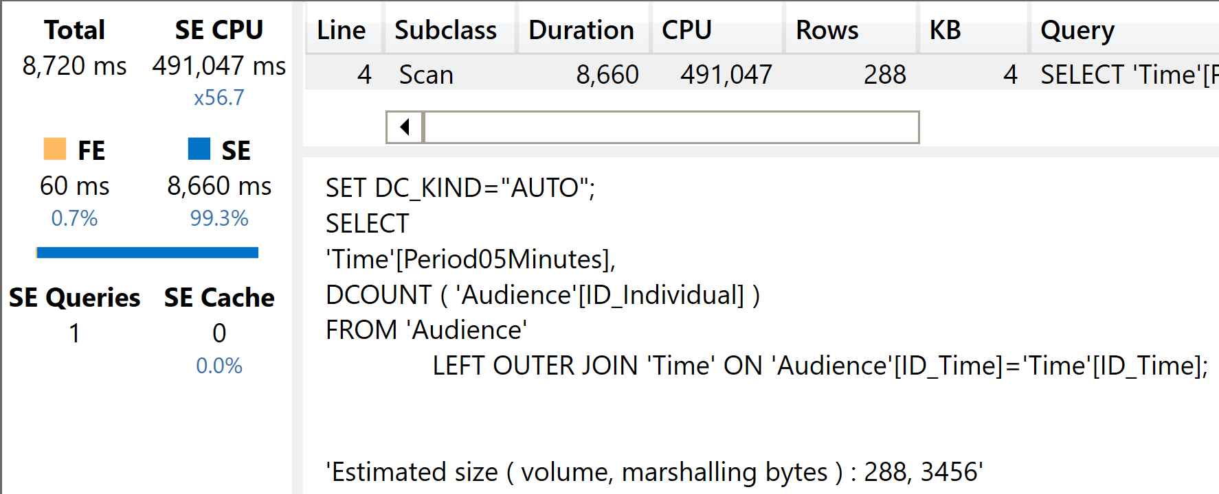
As you see, the storage engine CPU time increased by a lot, because a distinct count is much heavier to compute than a sum. There is a relationship involved, as you can see from the xmSQL query.
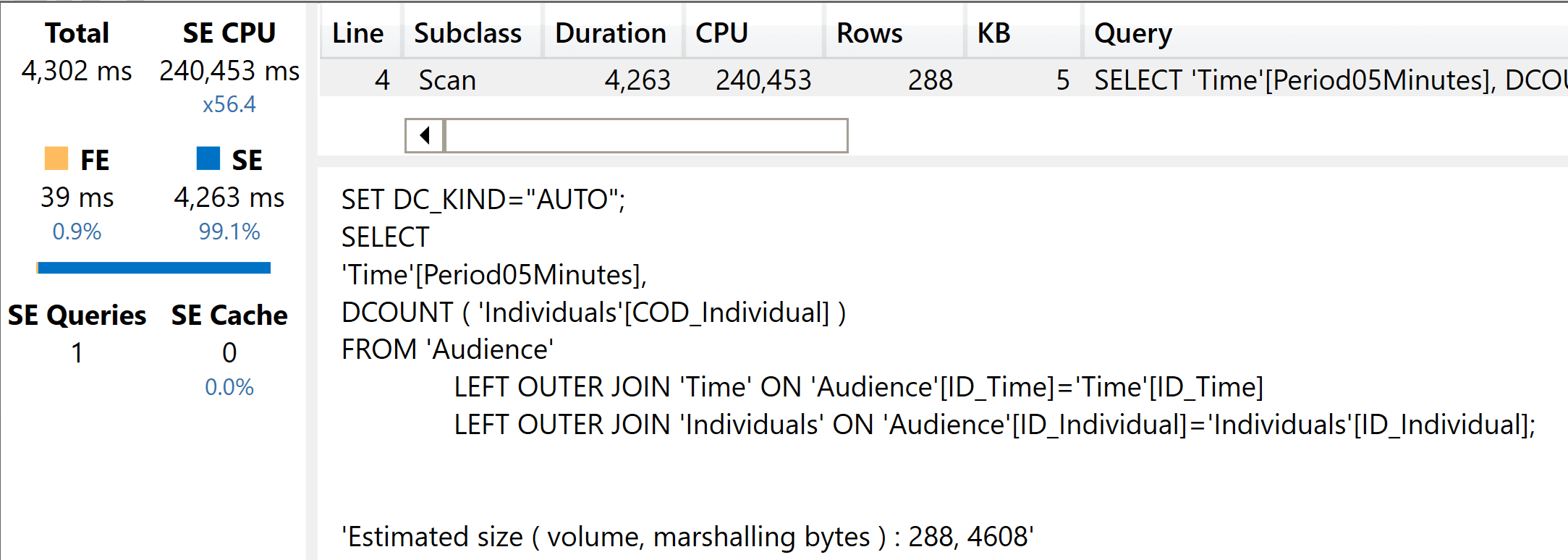
The same distinct count executed on the fat model requires this query:
EVALUATE
SUMMARIZECOLUMNS(
    Audience[Period05Minutes],
    "Test", DISTINCTCOUNT ( Audience[ID_Individual] )
)
The result is very similar to the slim model, exactly as we would have expected.

The xmSQL code shows that the relationship is no longer involved. That said, with a heavier calculation the impact of the relationship is lower. Indeed, this time the performance of the two queries is much closer than before.
The DAX query that computes a distinct count of COD_Individual in the fat model is very similar to the previous query. Indeed, both columns are stored in the fact table:
SUMMARIZECOLUMNS(
    Audience[Period05Minutes],
    "Weight", DISTINCTCOUNT ( Audience[COD_Individual] )
)
Because COD_Individual has fewer distinct values than ID_Individual, we expect better performance.
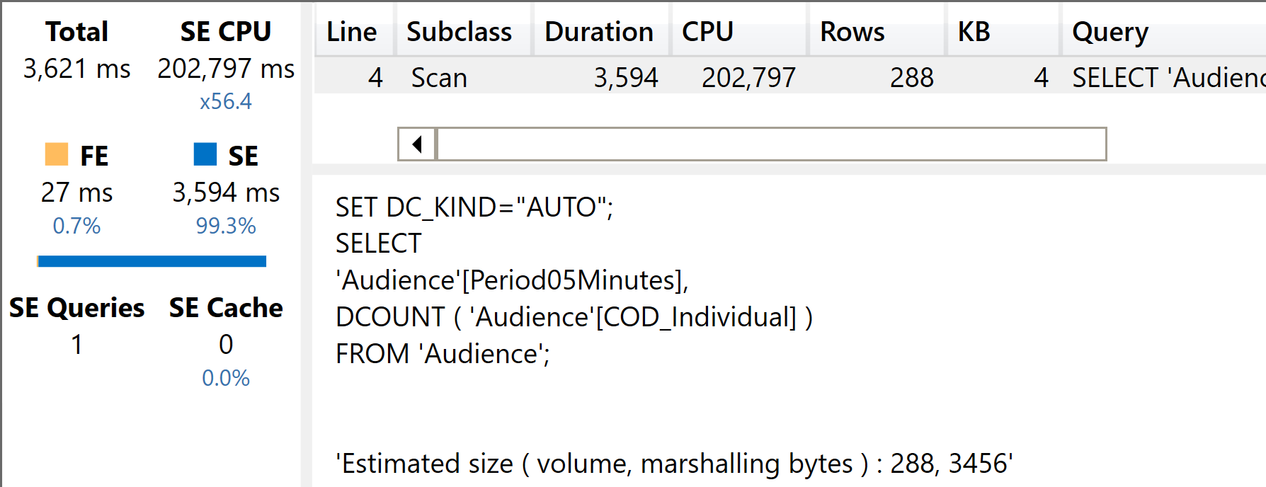
As you see, because the number of distinct values is smaller, this query runs at more than twice the speed of the previous one. This is totally expected: distinct counts strongly depend on the number of distinct values, that determines the size of internal structures used to perform the count.
On the slim model, the query needs to be different. We need to summarize the fact table by the column in the dimension – thus involving the relationship – and then count the number of values in the dimension filtered by the fact table:
EVALUATE
SUMMARIZECOLUMNS (
    Time[Period05Minutes],
    "Weight", COUNTROWS ( SUMMARIZE ( Audience, Individuals[COD_Individual] ) )
)
Despite this being more complex, the optimizer does a splendid job in finding an optimal execution plan.
In the slim model, DAX needs to traverse two relationships: one to perform the grouping and one to perform the counting. Despite the query being more complex, the optimizer found the optimal path. As expected the fat model is still a bit faster, but not by much.
So far, the conclusion we can draw is that the price of a relationship becomes less and less important depending on the complexity of the calculations involved. With very simple calculations, the relationship plays an important role in the total execution time. When the query becomes more complex, the relationship is no longer the heaviest part of the query and the differences between the two models start to become less and less important.
Distinct count grouping by multiple columns
Let us make the distinct count a bit more complex. We now want to compute the distinct count of COD_Individual, therefore involving the relationship with Individuals – but we increase the number of columns in the group by section.
This requires reading more large columns for the fat model, whereas the slim model needs to use a larger number of relationships. Therefore, we expect this query to be slower on both models. Let us start with the slim model. Here is the query:
EVALUATE
SUMMARIZECOLUMNS (
    'Date'[Year],
    'Date'[MonthNumber],
    Time[Period05Minutes],
    "Weight", COUNTROWS ( SUMMARIZE ( Audience, Individuals[Cod_Individual] ) )
)
As expected, the execution time is greater.
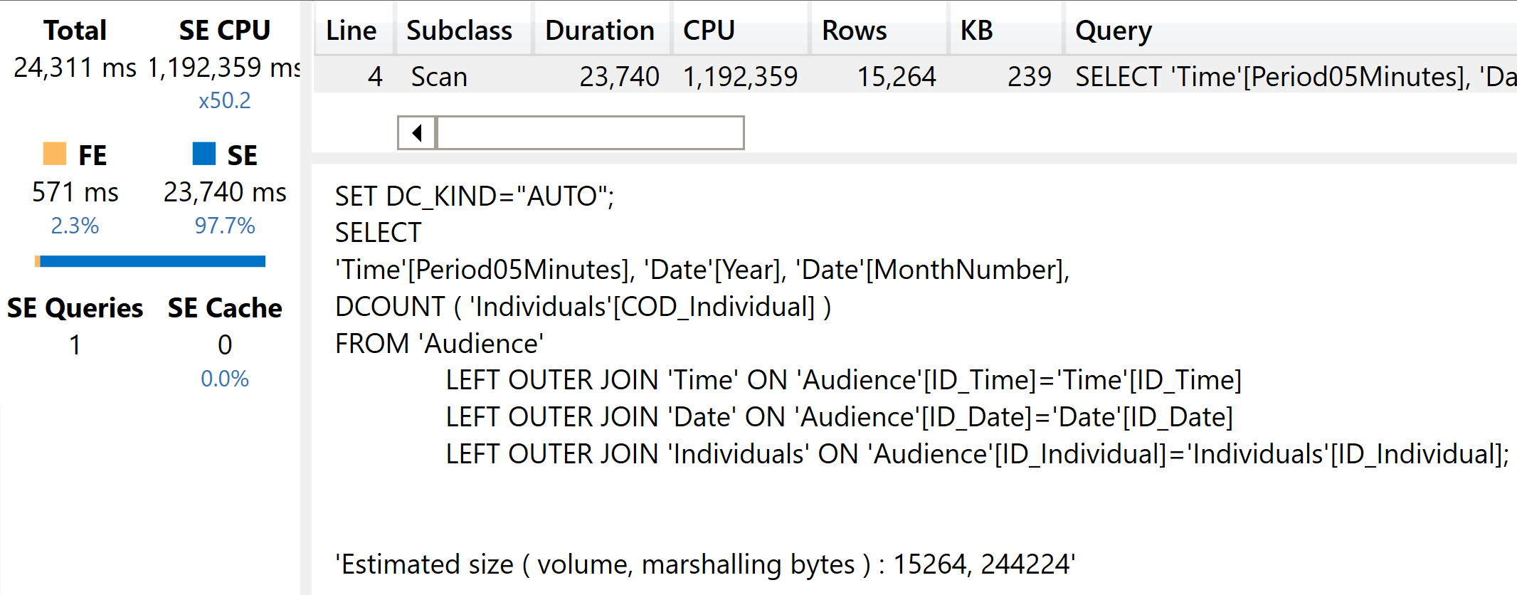
This time, with three relationships involved and more cells to compute the storage engine CPU went up to more than one million milliseconds.
The fat model does not require any relationship, but it needs to scan multiple large columns. Here is the query:
EVALUATE
SUMMARIZECOLUMNS (
    Audience[Period05Minutes],
    "Weight", DISTINCTCOUNT ( Audience[Cod_Individual] )
)
The size of the column weighs in here, as you can see from the results.
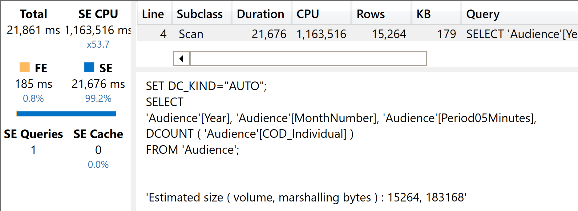
As clearly indicated by the xmSQL query, no relationships are involved. That said, the size of the columns and the complexity of the calculations also slowed down this query. We see an execution time very similar to the execution time of the slim model.
This is nothing but a confirmation of the previous findings. With simple calculations, the difference between the models determines a strong difference in terms of speed, and the fat model results being faster. With more complex queries, the model structure becomes less relevant and the difference between the two structures is neglectable. It is worth remembering that the fat model is much larger in terms of memory consumption than the slim one. Therefore, the price we pay in terms or RAM seems no longer justified by an increase in speed.
Year-to-date calculations
All the calculations we have shown so far were simply a SUM or a DISTINCTCOUNT that could be resolved with a single xmSQL query. Those queries were appropriate to measure the raw performance of the VertiPaq engine. However, a typical query involves work in both the formula engine (FE) and the storage engine (SE).
As an example, we use a simple year-to-date (YTD) calculation. Even there, it is interesting to investigate not only on the raw power of the engine, but also on the complexity of the code. Indeed, by using the slim model with a proper star schema, the year-to-date calculation could be expressed by leveraging the time intelligence functionalities of DAX:
Weight YTD =
    CALCULATE (
        SUM ( Audience[Weight] ),
        DATESYTD ( 'Date'[Date] ),
        ALL ( 'Date' )
    )
The same code would not work on the fat model, where there is no Date dimension. On the fat model the year-to-date needs to be written with custom DAX code, which implies more verbose and error-prone code. With that said we wanted to discuss performance here, not the simplicity of the DAX code. So we used the same complex calculation in both scenarios. What holds true is that a proper star schema makes the DAX code so much easier to write.
Here is the code we used for the YTD query on the slim model:
EVALUATE
SUMMARIZECOLUMNS (
    'Date'[Year],
    'Date'[MonthNumber],
    Time[Period05Minutes],
    "Weight",
        VAR YearStart =
            DATE ( MAX ( 'Date'[Year] ), 1, 1 )
        VAR CurrentDate =
            MAX ( 'Date'[Date] )
        VAR Result =
        CALCULATE (
            SUM ( Audience[Weight] ),
            'Date'[Date] >= YearStart && 'Date'[Date] <= CurrentDate,
            ALL ( 'Date' )
        )
        RETURN Result
)
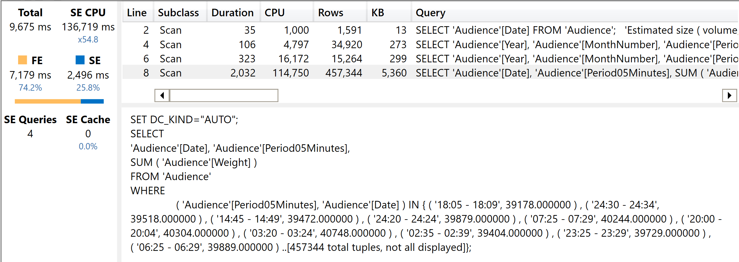
And here is the result of the execution. As you can see, there are now multiple storage engine queries and the formula engine starts to play a role.
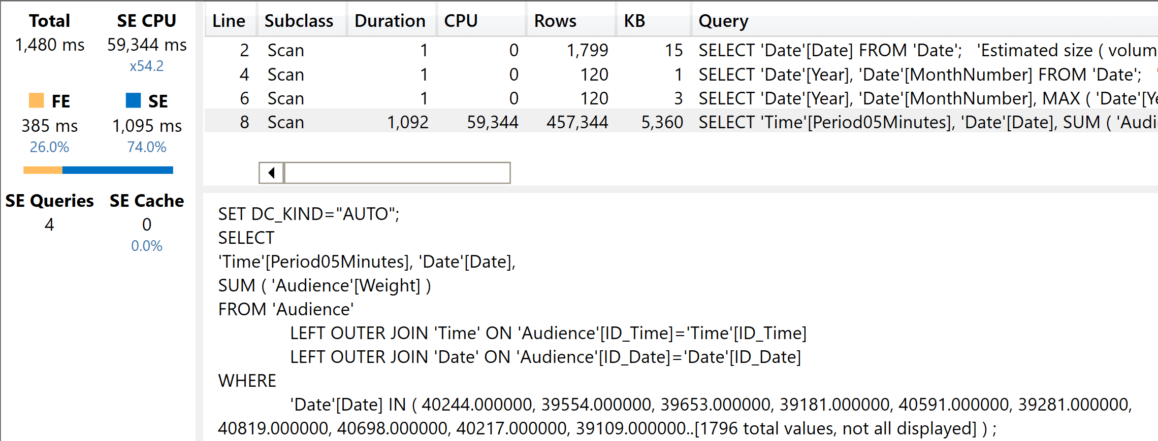
The main xmSQL query is rather fast. It retrieves the most granular data that is later aggregated by the formula engine, following the usual pattern of year-to-date. It is important to note that the filter on the xmSQL query includes only the date. The number of columns in the filter determines the size of the internal structures used to filter, and as such it determines the speed of the query. As you are going to see in the next query, with the fat model the xmSQL query is more complex. This results in poorer performance.
Here is the code executed on the fat table. As you see, the difference is only in the columns used:
EVALUATE
SUMMARIZECOLUMNS (
    'Audience'[Year],
    'Audience'[MonthNumber],
    'Audience'[Period05Minutes],
    "Weight",
        VAR YearStart =
            DATE ( MAX ( 'Audience'[Year] ), 1, 1 )
        VAR CurrentDate =
            MAX ( 'Audience'[Date] )
        VAR Result =
            CALCULATE (
                SUM ( Audience[Weight] ),
                Audience[Date] >= YearStart && 'Audience'[Date] <= CurrentDate,
                ALL ( Audience[MonthNumber] ),
                ALL ( Audience[Year] )
            )
        RETURN
            Result
)
This small difference – the columns used – turns out to be very relevant for the query plan. Because now all the columns come from the same table, auto-exist kicks in and the engine is forced to work with arbitrarily-shaped sets. Hence, the filter becomes more complex.
Now, as you see the filter contains not only the date but also Period05Minutes. The number of rows returned is the same, but the filter is much larger because DAX used arbitrarily-shaped sets during the evaluation. The net effect of this small detail is that the time is now more than twice what it was for the slim model.
The reason is not only in how VertiPaq scanned the data. The reason is that DAX is designed and optimized to work with star schemas. It assumes that a model resembles a star schema, and it uses specific optimizations that are efficient on star schemas and do not work well on flat models.
Values of a column
The last test we want to perform is extremely simple, yet very important. In a typical report, users place slicers and filters. Each slicer needs to retrieve the values of the column to show in the list. The resulting query is the simplest you can imagine: it just queries VALUES of the column.
On such a simple query, the difference between the slim and the fat model becomes huge. Indeed, the slim model can retrieve the values of a column from the dimension, whose size is tiny compared with the fact table. The fat model on the other hand always needs to scan the fact table, because all the columns are stored in there. For example, in order to retrieve the ten values for the Year column the fat model scans four billion rows!
In a typical report you would find tens of these small queries. Therefore, simple queries need to be very fast, otherwise they tend to steal CPU time away from the more complex matrices and calculations.
Let us look at two versions of VALUES: one without any filter, and one with a filter. Again, the reason is that slicers and tables might be cross-filtered. If you place one slicer for the customer country and one slicer for the time period, they cross-filter each other because they belong to the same table.
Here is the first query:
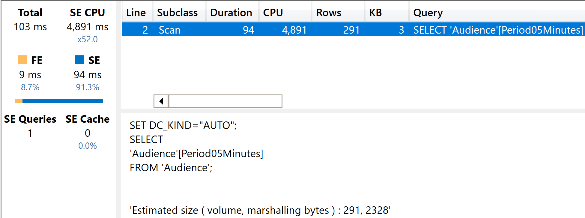
EVALUATE
    VALUES ( Audience[Period05Minutes] )
As you see, the result is an incredible five seconds of CPU time. Because of the high level of parallelism, the execution time is very fast. Still, the CPU was used heavily.
The presence of a cross-filter makes things even worse. Here is a filtered VALUES query on the fat model:
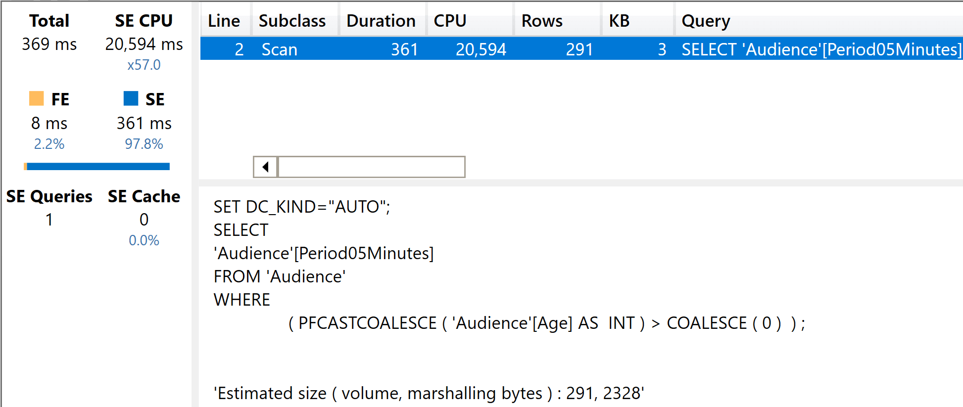
EVALUATE
    CALCULATETABLE(
        VALUES ( Audience[Period05Minutes] ),
        Audience[Age] > 0
    )
The presence of the filter made the simple VALUES query run four times more slowly.
This last test is extremely important: with a fat model, any filter on any column results in a filter over the fact table. Therefore, you obtain a nice cross-filtering effect. Nice for the users, still extremely heavy on the CPU.
The same queries executed on the slim model result in zero or 1 millisecond of execution time. This is because the slim model needs to scan a dimension, not the fact table. Each dimension contains a few thousand rows, which is nothing compared to the billions present in the fact table.
Conclusions
We performed several interesting tests on the slim model versus the fat model. The results are synthetized in an Excel report below.
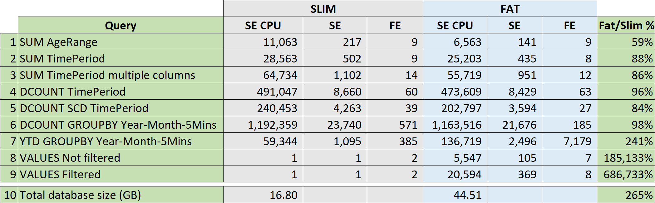
As you see from the results, the fat model is indeed faster with extremely simple queries. As soon as the query increases in complexity, the benefits of the fat model fade away very quickly. If the query is not a pure SE query, the slim model performs much better. When it comes to retrieving values for columns in slicers, the fat model is extremely slow. The important takeaway here is the following: when the fat model is better, it is not that much better. When it is worse, it is far worse!
From a memory consumption point of view, the fat model is three times the size of the slim model. In other words, you need to spend more either on on-premises servers or on cloud services to manage the fat model.
In conclusion, by going towards a single table model you obtain a larger model that performs slightly better on a limited number of simple queries, but becomes terribly slow as soon as the query increases in complexity.
I dare to conclude that apart from an extremely limited number of scenarios where you need to super-optimize specific calculations, the fat model proves to be the worst option for a Tabular model.
The next time a zealous consultant suggests that you build a single fat table for your data model, you know what to do: measure the performance and evaluate the additional cost – or simply point to this article to start the discussion with supporting numbers!
Adds all the numbers in a column.
SUM ( <ColumnName> )
Counts the number of distinct values in a column.
DISTINCTCOUNT ( <ColumnName> )
When a column name is given, returns a single-column table of unique values. When a table name is given, returns a table with the same columns and all the rows of the table (including duplicates) with the additional blank row caused by an invalid relationship if present.
VALUES ( <TableNameOrColumnName> )