 Marco Russo & Alberto Ferrari
Let us state this from the very beginning: context transition is a simple concept. It is a powerful feature aiming to simplify the authoring of DAX code. That said, most new DAX developers find context transition hard to understand, and they consider it to be the major reason behind incorrect results. There are two reasons for developers to feel this way:
- A solid understanding of the difference between the row context and the filter context is an important prerequisite to understand and master the concept of context transition.
- You need to remember when and how the context transition works. Most errors involving context transition are due to the developer forgetting to take the context transition into account, rather than not knowing how it works. Once they realize that context transition is happening, the code suddenly makes sense.
These two factors are not a peculiarity of the context transition. They are relevant in almost every aspect of DAX. DAX requires you to remember details and understand the fundamentals well.
If you are not familiar with the row context and the filter context, we suggest you read and understand really well the two previous articles:
Nonetheless, this short introduction is important to understand the definition of context transition. Here is its definition:
CALCULATE triggers context transition.
Context transition transforms any existing row context into an equivalent filter context,
which is then used by CALCULATE to evaluate its first argument.
If you are not familiar with the row context and the filter context, their differences and their behaviors, then the previous definition does not mean much. Indeed, the context transition is the transformation of a row context into a filter context. This is why you need to know the differences between the two evaluation contexts very well, to better appreciate what the transformation of one into the other implies.
Context transition happens when CALCULATE (or CALCULATETABLE) is executed inside a row context. Sometimes this is easy to spot, whereas sometimes one of the two prerequisites for the context transition is somewhat hidden and harder to see. Let us elaborate a bit:
- First, context transition is invoked by CALCULATE. If CALCULATE is not present in your code, then there is no context transition. Be mindful that CALCULATE is always present when you invoke a measure; therefore a context transition might occur when you call a measure, without any explicit CALCULATE in your code.
- Second, context transition requires the presence of a row context. If there is no row context, then no context transition happens, because there would be no row context to transform. The row context can be explicitly introduced with an iterator, but it might also be present because you are writing code in a calculated column – where by default, there is a row context.
Let us show two examples where the context transition is entirely explicit, or entirely implicit. First, let us look at an example where the presence of context transition is evident with a measure that computes the sales to big customers:
Sales to big customers :=
SUMX (
    VALUES ( Customer[CustomerKey] ),
    VAR CustomerSales =
        CALCULATE (
            SUMX ( Sales, Sales[Quantity] * Sales[Net Price] )
        )
    VAR Result = IF ( CustomerSales >= 5000, CustomerSales )
    RETURN
        Result
)
In this measure, context transition happens during the evaluation of the CustomerSales variable. There is a row context introduced by SUMX iterating over Customer and an explicit invocation of CALCULATE. Therefore, the prerequisites for context transition are present and the row context over VALUES ( Customer[CustomerKey] ) is transformed into a filter context, so that the inner SUMX is executed in a filter context showing only the current customer key.
The prerequisites for context transition are easy to spot in that code. We have not yet discussed what context transition does in detail; at least we understood when it may happen. What makes the phenomenon of context transition challenging is the presence of the prerequisites in scenarios where they are very well hidden. Let us look at the next piece of DAX code, which is a calculated column in Customer:
Sales = [Sales Amount]
This time, the expression is a simple measure called from inside a calculated column. Context transition is happening: the prerequisites are all there, just very well hidden. There is a row context because the code is that of a calculated column, and calculated columns are computed in an implicit row context over the table where they are defined. The code invokes the Sales Amount measure; whenever a measure is invoked, it is automatically surrounded by CALCULATE. Hence, the measure is evaluated after the hidden CALCULATE has performed the context transition.
This last example looks surprisingly simple, yet it already shows the trap of context transition. Finding the combination of row context and CALCULATE in more complex formulas might be more difficult. Nonetheless, the rule is simple: when both the row context and CALCULATE happen to be together, then they trigger the context transition. Getting used to finding the combination may take some time, but it is one of many important skills for a good DAX developer.
Now that we have clarified when the context transition takes place, it is time to dig more into the effect of context transition. Context transition transforms the row context into an equivalent filter context. The new filter context created by the context transition includes all the columns currently being iterated by the row context. It filters these columns with the value of the current row. If the row context is iterating one column only, then that column will be part of the filter context. If the row context is iterating over an entire table, then all the columns of the table will be part of the newly-created filter context. Actually, all the columns of the expanded table will be part of the newly-created filter context. But we do not want to make things more complex by introducing expanded tables, therefore we avoid this detail in this more introductory article.
Let us look at the measure we saw previously:
Sales to big customers :=
SUMX (
    VALUES ( Customer[CustomerKey] ),
    VAR CustomerSales =
        CALCULATE (
            SUMX ( Sales, Sales[Quantity] * Sales[Net Price] )
        )
    VAR Result = IF ( CustomerSales >= 5000, CustomerSales )
    RETURN
        Result
)
The context transition is happening in the rows that are highlighted. Because the row context is iterating a table containing only Customer[CustomerKey], CALCULATE applies a filter to the Customer[CustomerKey] column automatically. The code is equivalent to the following formulation, where we made the filter on the Customer[CustomerKey] column explicit:
Sales to big customers :=
SUMX (
    VALUES ( Customer[CustomerKey] ),
    VAR CurrentCustomerKey = Customer[CustomerKey]
    VAR CustomerSales =
        CALCULATE (
            SUMX ( Sales, Sales[Quantity] * Sales[Net Price] ),
            Customer[CustomerKey] = CurrentCustomerKey
        )
    VAR Result = IF ( CustomerSales >= 5000, CustomerSales )
    RETURN
        Result
)
As you see, we saved the current value of the Customer[CustomerKey] column in the CurrentCustomerKey variable and we then used it as an explicit filter inside CALCULATE.
It is very common for newbies to think that because we are iterating over Customer[CustomerKey], the column is already filtered. This is not correct. The row context iterates a table, it does not place any filter on the current value. Without CALCULATE and the context transition, there would be no active filter on Customer[CustomerKey]. Remember: the row context iterates, it does not filter. The only evaluation context that applies a filter is the filter context. By transforming the row context into a filter context, we can create a filter context that filters the values being iterated by the row context.
The example we have shown is quite simple, as the table iterated contained only one column. In the case of a calculated column, the scenario is more complex. The reason is that the context transition is happening in a row context that includes the entire table. Therefore, all the columns of the Customer table are part of the new filter context. This is the original calculated column:
Sales = [Sales Amount]
When the context transition happens, all the columns in Customer get filtered. This is the equivalent code using variables to make the filter explicit:
Sales =
VAR CurrentAddress      = Customer[Address]
VAR CurrentAge          = Customer[Age]
VAR CurrentBirthday     = Customer[Birthday]
VAR CurrentCity         = Customer[City]
VAR CurrentContinent    = Customer[Continent]
VAR CurrentCountry      = Customer[Country]
VAR CurrentCountryCode  = Customer[Country Code]
VAR CurrentCustomerKey  = Customer[CustomerKey]
VAR CurrentGender       = Customer[Gender]
VAR CurrentName         = Customer[Name]
VAR CurrentState        = Customer[State]
VAR CurrentStateCode    = Customer[State Code]
VAR CurrentZipCode      = Customer[Zip Code]
RETURN
    CALCULATE (
        [Sales Amount],
        Customer[Address]      = CurrentAddress,
        Customer[Age]          = CurrentAge,
        Customer[Birthday]     = CurrentBirthday,
        Customer[City]         = CurrentCity,
        Customer[Continent]    = CurrentContinent,
        Customer[Country]      = CurrentCountry,
        Customer[Country Code] = CurrentCountryCode,
        Customer[CustomerKey]  = CurrentCustomerKey,
        Customer[Gender]       = CurrentGender,
        Customer[Name]         = CurrentName,
        Customer[State]        = CurrentState,
        Customer[State Code]   = CurrentStateCode,
        Customer[Zip Code]     = CurrentZipCode
    )
As you see, the context transition retrieves the current value of each column present in the row context; it uses that value as an explicit filter to create a filter context, under which it evaluates its first argument.
This first example shows that when a context transition takes place during an iteration over a full table, it is much more expensive than when it takes place over a table containing only one column. The more columns in the table, the more time needed for the context transition.
It is important to note that in this last example what causes the context transition is the hidden CALCULATE surrounding each measure reference. Indeed, if we replace the measure reference with the code of the measure itself, then the scenario is very different. Look at the following code:
Sales Amount :=
SUMX ( Sales, Sales[Quantity] * Sales[Net Price] )
Sales 1 =
[Sales Amount]
Sales 2 =
SUMX ( Sales, Sales[Quantity] * Sales[Net Price] )
The Sales 1 column is the same code as in the previous example, whereas the Sales 2 column uses the internal expression of Sales Amount instead of referencing the Sales Amount measure. Despite looking the same, the two columns are actually very different.
Sales 1 uses a measure reference, therefore there is a context transition there. Both the row context and CALCULATE are present, albeit hidden. In Sales 2, there is a row context but CALCULATE is missing. Therefore, no context transition is taking place. The result of Sales 2 is the amount of sales to all customers, whereas the result of Sales 1 is the amount of sales to the current customer only. Remember that the presence of a row context does not imply any filtering. The row context only iterates a table.
At this point we have observed that the complexity of context transitions lies not in the operation itself, but rather in our ability to spot when the transition does and does not occur. Most developers who start to use DAX find it very hard to distinguish for example between these two versions of a running total measure:
MaxDate :=
MAX ( 'Date'[Date] )
RT Sales 1 :=
CALCULATE (
    [Sales Amount],
    FILTER (
        ALL ( 'Date' ),
        'Date'[Date] <= [MaxDate]
    )
)
RT Sales 2 :=
CALCULATE (
    [Sales Amount],
    FILTER (
        ALL ( 'Date' ),
        'Date'[Date] <= MAX ( 'Date'[Date] )
    )
)
As a matter of fact, the two measures return a very different result.
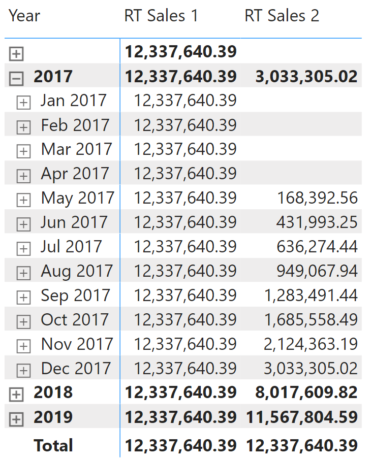
As you see, RT Sales 1 returns the grand total of sales in every cell, whereas RT Sales 2 produces a running total of the sales amount. The difference between the two is only that RT Sales 2 uses MAX directly inside FILTER, whereas RT Sales 1 invokes a measure.
Because RT Sales 1 invokes a measure, we know that CALCULATE is there. In both cases, when we compute the maximum date, we are computing it inside an iteration over ALL ( Date ). When the context transition occurs, the measure is executed in a filter context that is filtering the iterated date, always returning the currently iterated date. Because each date is less or equal to itself, the FILTER function returns the entire Date table: it shows the grand total in every cell. In RT Sales 2, on the other hand, MAX is executed without a CALCULATE around it. So it computes the max date in the outer filter context, created by the visual through SUMMARIZECOLUMNS. As such, it computes the last visible date in the visual, and produces the correct result.
Conclusions
In this article we just scratched the surface of context transition. Context transition in itself is not a complex topic. What makes context transition complex to master is that it is oftentimes hard to spot because of the automatic CALCULATE present for measures. Moreover, the complexity for a good DAX developer is real as they would have to keep in mind the possibility of context transition – on top of many other details – as they author their code. DAX is not forgiving: many small details have to be taken into account, each of which might change the result of your code. Learning DAX requires you to slow down, learn the fundamentals the right way and slowly proceed from rookie to master.
If you want to learn more, then start by watching the free Introducing DAX video course. Once you have digested that content, proceed with one of our in-person classroom courses and/or with watching the Mastering DAX online video course.
Evaluates an expression in a context modified by filters.
CALCULATE ( <Expression> [, <Filter> [, <Filter> [, … ] ] ] )
Evaluates a table expression in a context modified by filters.
CALCULATETABLE ( <Table> [, <Filter> [, <Filter> [, … ] ] ] )
Returns the sum of an expression evaluated for each row in a table.
SUMX ( <Table>, <Expression> )
When a column name is given, returns a single-column table of unique values. When a table name is given, returns a table with the same columns and all the rows of the table (including duplicates) with the additional blank row caused by an invalid relationship if present.
VALUES ( <TableNameOrColumnName> )
Returns the largest value in a column, or the larger value between two scalar expressions. Ignores logical values. Strings are compared according to alphabetical order.
MAX ( <ColumnNameOrScalar1> [, <Scalar2>] )
Returns a table that has been filtered.
FILTER ( <Table>, <FilterExpression> )
Returns all the rows in a table, or all the values in a column, ignoring any filters that might have been applied.
ALL ( [<TableNameOrColumnName>] [, <ColumnName> [, <ColumnName> [, … ] ] ] )
Create a summary table for the requested totals over set of groups.
SUMMARIZECOLUMNS ( [<GroupBy_ColumnName> [, [<FilterTable>] [, [<Name>] [, [<Expression>] [, <GroupBy_ColumnName> [, [<FilterTable>] [, [<Name>] [, [<Expression>] [, … ] ] ] ] ] ] ] ] ] )
Articles in the DAX 101 series
- Computing running totals in DAX
- Counting working days in DAX
- Summing values for the total
- Year-to-date filtering weekdays in DAX
- Creating a simple date table in DAX
- Automatic time intelligence in Power BI
- Using CONCATENATEX in measures
- Previous year up to a certain date
- Sorting months in fiscal calendars
- Using USERELATIONSHIP in DAX
- Mark as Date table
- Row context in DAX
- Filter context in DAX
- Introducing CALCULATE in DAX
- Understanding context transition in DAX
- Using KEEPFILTERS in DAX
- Variables in DAX
- Using RELATED and RELATEDTABLE in DAX
- Introducing ALLSELECTED in DAX
- Introducing RANKX in DAX