 Marco Russo & Alberto Ferrari
A common requirement in reporting is the ability to compare different time periods. For example, you might need a report like the following one.
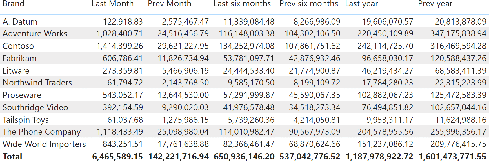
On the columns we see different time periods, which can be compared in pairs (Last vs. Prev). The last month overall, versus the previous month; the last six months against the six previous months and the same for the last year. The user has the option of choosing a time period, so that calculations refer to that period. Moreover, the selection is dynamic: as soon as the data is refreshed, the time periods adjust themselves to always refer to the most current “last month”.
There are multiple options to solve that scenario. The most commonly used options are calculation groups, or a bridge table between the time periods and the Date dimension – this is to be able to use time periods to filter dates. Both scenarios have advantages and disadvantages. In this article we perform a comparison of the two techniques, briefly describing how they work and then comparing the performance of the two options.
Using calculation groups
Solving the scenario through calculation groups is rather simple: we just have to create one calculation item for each time period where the calculation item uses SELECTEDMEASURE and a mix of time intelligence calculations to provide the result:
---------------------------------
-- Calculation Group: 'Period CG'
---------------------------------
CALCULATIONGROUP 'Period CG'[Period CG]

    CALCULATIONITEM "Last Month" =
        VAR MaxDate = CALCULATE ( MAX ( Sales[Order Date] ), REMOVEFILTERS () )
        RETURN
            CALCULATE (
                SELECTEDMEASURE ( ),
                DATESBETWEEN (
                    'Date'[Date],
                    EOMONTH ( MaxDate, -1 ) + 1,
                    EOMONTH ( MaxDate, 0 )
                )
            )
        Ordinal = 0

    CALCULATIONITEM "Prev Month" =
        VAR MaxDate = CALCULATE ( MAX ( Sales[Order Date] ), REMOVEFILTERS () )
        RETURN
            CALCULATE (
                SELECTEDMEASURE ( ),
                DATESBETWEEN (
                    'Date'[Date],
                    EOMONTH ( MaxDate, -2 ) + 1,
                    EOMONTH ( MaxDate, -1 )
                )
            )
        Ordinal = 1

    CALCULATIONITEM "Last 6 Months" =
        VAR MaxDate = CALCULATE ( MAX ( Sales[Order Date] ), REMOVEFILTERS () )
        RETURN
            CALCULATE (
                SELECTEDMEASURE ( ),
                DATESBETWEEN (
                    'Date'[Date],
                    EOMONTH ( MaxDate, -6 ) + 1,
                    EOMONTH ( MaxDate, 0 )
                )
            )
        Ordinal = 2

    CALCULATIONITEM "Prev 6 Months" =
        VAR MaxDate = CALCULATE ( MAX ( Sales[Order Date] ), REMOVEFILTERS () )
        RETURN
            CALCULATE (
                SELECTEDMEASURE ( ),
                DATESBETWEEN (
                    'Date'[Date],
                    EOMONTH ( MaxDate, -12 ) + 1,
                    EOMONTH ( MaxDate, -6 )
                )
            )
        Ordinal = 3

    CALCULATIONITEM "Last Year" =
        VAR MaxDate = CALCULATE ( MAX ( Sales[Order Date] ), REMOVEFILTERS () )
        RETURN
            CALCULATE (
                SELECTEDMEASURE ( ),
                DATESBETWEEN (
                    'Date'[Date],
                    EOMONTH ( MaxDate, -12 ) + 1,
                    EOMONTH ( MaxDate, 0 )
                )
            )
        Ordinal = 4

    CALCULATIONITEM "Prev Year" =
        VAR MaxDate = CALCULATE ( MAX ( Sales[Order Date] ), REMOVEFILTERS () )
        RETURN
            CALCULATE (
                SELECTEDMEASURE ( ),
                DATESBETWEEN (
                    'Date'[Date],
                    EOMONTH ( MaxDate, -24 ) + 1,
                    EOMONTH ( MaxDate, -12 )
                )
            )
        Ordinal = 5
Despite being long, this calculation group definition is rather simple: each calculation item uses a different filter over the Date table, finding the proper set of dates that produces the required result. Every calculation item uses MaxDate to find the reference date in the Sales table – to in turn, obtain a dynamic calculation.
Using many-to-many relationships
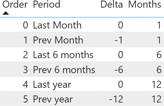
The solution with many-to-many relationships requires adding two tables to the model. The first table is a configuration table, where we define the time periods with two columns: Delta and Months. Delta is the number of months to travel back, using the max date as the reference; Months is the duration of the time period.
Based on this configuration table, we create a new calculated table that uses the configuration to create a bridge table that states which dates need to be used for each period:
Period =
VAR RefDate = MAX ( Sales[Order Date] )
RETURN
    SELECTCOLUMNS (
        GENERATE (
            'Period Config',
            VAR DateStart = EOMONTH ( RefDate, 'Period Config'[Delta] - 'Period Config'[Months] ) + 1
            VAR DateEnd = EOMONTH ( RefDate, 'Period Config'[Delta] )
            RETURN
                DATESBETWEEN ( 'Date'[Date], DateStart, DateEnd )
        ),
        "Date", 'Date'[Date],
        "Period", 'Period Config'[Period],
        "Order", 'Period Config'[Order]
    )
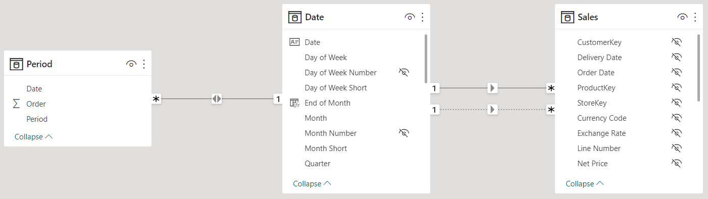
The resulting table needs to be linked to Date through a bidirectional relationship so that a filter on Period is propagated first to Date, and then to Sales.
There is no need to author DAX code in this scenario. The filter propagation happens automatically; therefore, all measures are affected by the change in the model.
Comparing maintenance and flexibility
From a maintenance point of view, the differences are rather small. The calculation group solution is extremely flexible, because each calculation item is defined through DAX code: creating new time periods is a simple task.
For example, to add new periods for the last and previous weeks, the calculation group solution is straightforward and requires the deployment of a new version of the data model. The many-to-many solution requires changes to the configuration table structure to accommodate a different period granularity. Adding periods based on a whole number of months is easy, whereas changing the granularity to weeks or days proves to be more challenging. On the other hand, as long as there are no changes in the granularity of the definition, adding new periods to the many-to-many solution is actually simpler. Updating the configuration table is enough, and the entire model adapts itself to the new periods.
Therefore, the calculation group solution is slightly more flexible, but at the same time it requires writing DAX code every time you add a new time period. The many-to-many solution is slightly less flexible, but it saves you from writing DAX code, as long as the grain of the configuration table supports the definition of the new periods.
Comparing performance
Maintenance and flexibility are important factors, but the most relevant aspect to check is undoubtedly performance. Before we move forward, let us make several considerations.
The solution based on the calculation group uses DATESBETWEEN. DATESBETWEEN, like all time intelligence functions, is resolved in the formula engine. Therefore, whenever you use DATESBETWEEN in the code, there will be several steps: the formula engine will retrieve the dates from the Date table, then it will compute the filter needed by DATESBETWEEN to identify the set of dates to query, and finally it will execute a storage engine query to retrieve the results. The storage engine query will directly filter the dates based on the filter set on Date.
The solution based on many-to-many relationships uses an entirely different algorithm. The period table is filtered by the user. This determines a set of dates to filter Date through the bidirectional filter. Past this point, the filter goes to Sales through regular relationships. With bidirectional relationships, the price of the filter strongly depends on the size of the intermediate structures created by VertiPaq to move the filters. Usually, bidirectional relationships are slow. Nonetheless, they have the advantage of being resolved entirely in the storage engine and – in our scenario – the size of the filtering structure is very small, because it consists of a few hundred rows.
Now that we have a rough idea of what to expect, we can perform a few measurements. Be mindful of the fact that any result we describe is based on our specific data model, with our data distribution. It is likely your model will be different. Therefore, never take for granted that our conclusions apply to your calculations in a straightforward manner. You always need to perform the test again on your system before making an educated choice.
The difference in terms of speed is almost irrelevant, whereas the algorithm followed by the two solutions is very different in case we are using additive calculations. With non-additive calculations, the two algorithms become surprisingly close.
Let us first run a query with all the different periods, slicing by columns in Customer, Store and Product:
EVALUATE
    SUMMARIZECOLUMNS (
        'Product'[Brand],
        Customer[Country],
        Customer[Gender],
        Store[Name],
        Period[Period],
        Period[Order],
        "Sales Amount", [Sales Amount]
    )
The query runs quite fast, with a single VertiPaq query consisting of a batch.
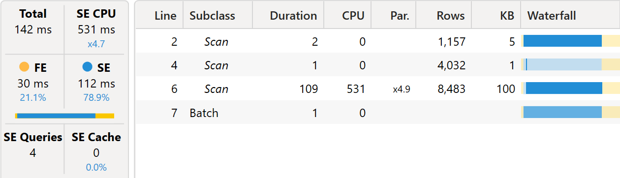
The batch executes the entire calculation in a single xmSQL query:
DEFINE TABLE '$TTable3' :=
SELECT
    'Date'[Date],
    'Table'[Period],
    'Table'[Order]
FROM 'Table'
    LEFT OUTER JOIN 'Date' ON 'Table'[Date]='Date'[Date],

DEFINE TABLE '$TTable4' :=
SELECT
    SIMPLEINDEXN ( '$TTable3'[Date$Date] )
FROM
    '$TTable3',

CREATE SHALLOW RELATION '$TRelation1' MANYTOMANY FROM 'Date'[Date] TO '$TTable3'[Date$Date],

DEFINE TABLE '$TTable1' :=
SELECT
    '$TTable2'[Customer$Gender],
    '$TTable2'[Customer$Country],
    '$TTable2'[Product$Brand],
    '$TTable2'[Store$Name],
    '$TTable3'[Table$Period],
    '$TTable3'[Table$Order],
    SUM ( '$TTable2'[$Measure0] )
FROM '$TTable2'
    INNER JOIN '$TTable3'
        ON '$TTable2'[Date$Date]='$TTable3'[Date$Date]
    REDUCED BY
        '$TTable2' :=
            WITH
                $Expr0 := (
                      PFCAST ( 'Sales'[Quantity] AS  INT ) *
                      PFCAST ( 'Sales'[Net Price] AS  INT )
                 )
            SELECT
                'Customer'[Gender],
                'Customer'[Country],
                'Date'[Date],
                'Product'[Brand],
                'Store'[Name],
                SUM ( @$Expr0 )
            FROM 'Sales'
                LEFT OUTER JOIN 'Customer' ON 'Sales'[CustomerKey]='Customer'[CustomerKey]
                LEFT OUTER JOIN 'Date' ON 'Sales'[Order Date]='Date'[Date]
                LEFT OUTER JOIN 'Product' ON 'Sales'[ProductKey]='Product'[ProductKey]
                LEFT OUTER JOIN 'Store' ON 'Sales'[StoreKey]='Store'[StoreKey]
            WHERE
                'Date'[Date] ININDEX '$TTable4'[$SemijoinProjection];
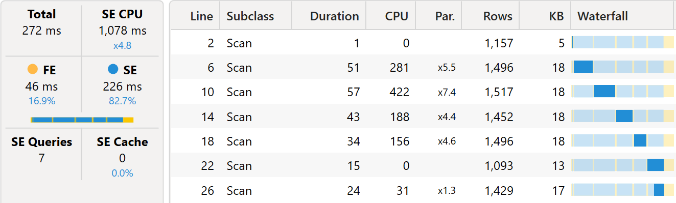
Confirming the simplicity of the solution, the query plan is the simplest one could imagine.
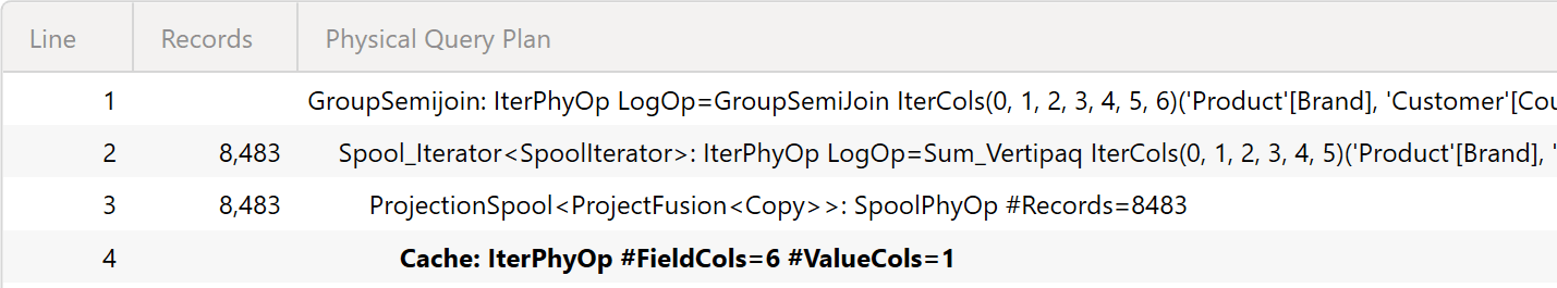
The level of materialization is just perfect: the result set contains 8,483 rows. That is exactly the number of rows materialized by the VertiPaq engine.
The same query shows a different behavior when using the calculation groups:
EVALUATE
    SUMMARIZECOLUMNS (
        'Product'[Brand],
        Customer[Country],
        Customer[Gender],
        Store[Name],
        'Period CG'[Period CG],
        'Period CG'[Ordinal],
        "Sales Amount", [Sales Amount]
    )
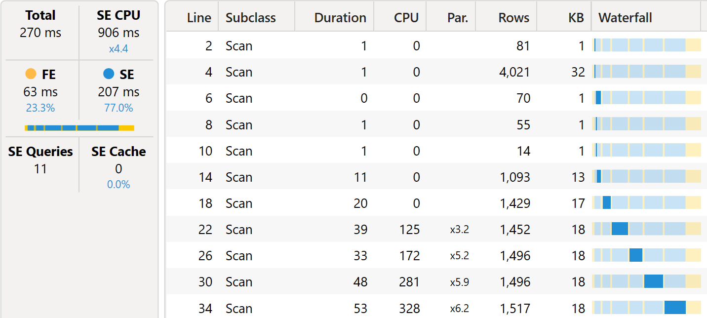
Despite the timings being nearly identical, there are many more VertiPaq queries, interleaved by short burst of the formula engine.
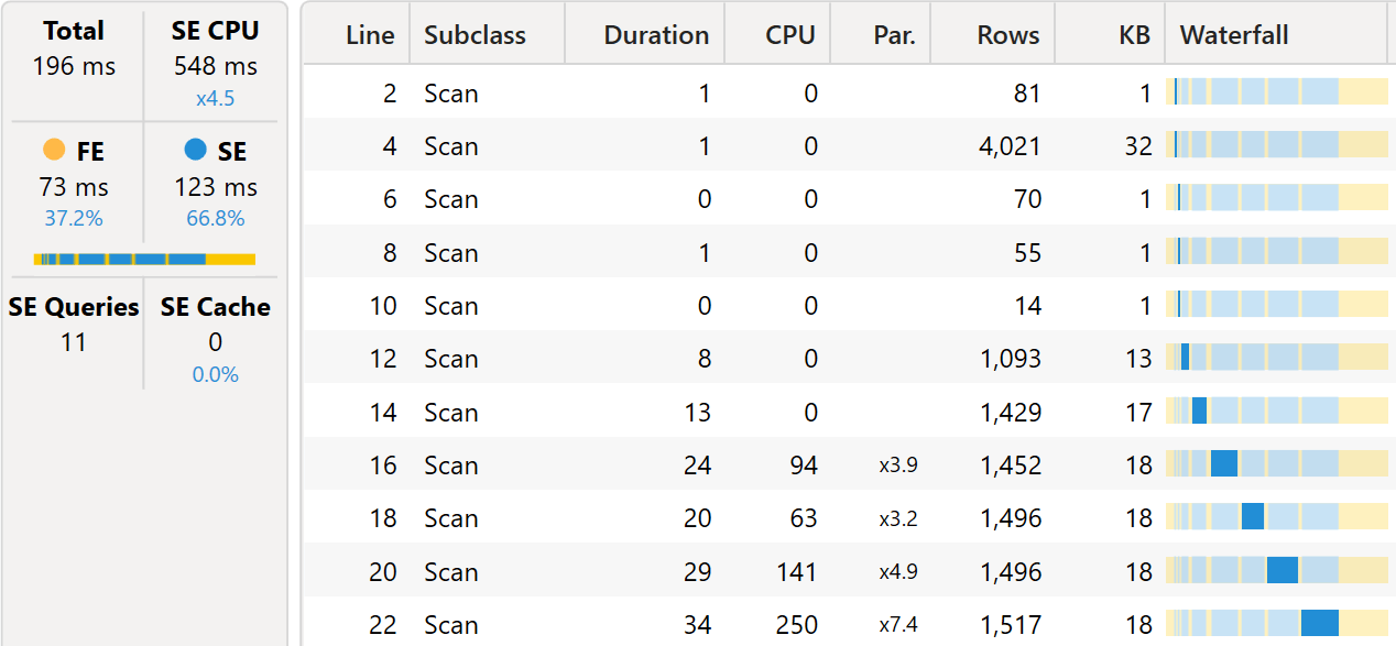
The first set of very short queries retrieves the values of the columns. At line 4, there is a VertiPaq query retrieving the dates from the Date table. This table is then used by the formula engine to solve the DATESBETWEEN calculations, that determine the filters of the next (longer) queries from line 12 on. These queries all have the same shape, despite having different filters:
WITH
    $Expr0 := ( PFCAST ( 'Sales'[Quantity] AS  INT ) * PFCAST ( 'Sales'[Net Price] AS  INT )  )
SELECT
    'Customer'[Gender],
    'Customer'[Country],
    'Product'[Brand],
    'Store'[Name],
    SUM ( @$Expr0 )
FROM 'Sales'
    LEFT OUTER JOIN 'Customer' ON 'Sales'[CustomerKey]='Customer'[CustomerKey]
    LEFT OUTER JOIN 'Date' ON 'Sales'[Order Date]='Date'[Date]
    LEFT OUTER JOIN 'Product' ON 'Sales'[ProductKey]='Product'[ProductKey]
    LEFT OUTER JOIN 'Store' ON 'Sales'[StoreKey]='Store'[StoreKey]
WHERE
    'Date'[Date] IN (
        43868.000000, 43881.000000, 43882.000000, 43869.000000, 43883.000000,
        43870.000000, 43884.000000, 43871.000000, 43885.000000, 43872.000000
        ..[29 total values, not all displayed]
    ) ;
There is one of those VertiPaq queries per calculation item.
The difference between the two algorithms is not entirely evident with small databases. In our tests, we use a model with 10 million rows in Sales. Therefore, the degree of parallelism is limited and the strong difference between the formula engine and the storage engine does not come into play.
The same queries show a noticeable difference when executed on a model with 1.4 billion rows. First, the version with calculation groups.
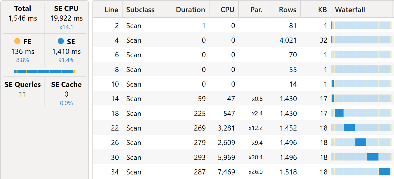
As you see, there are several small VertiPaq queries, each of which cannot reach a good degree of parallelism. Therefore, the server is underused.
The query using the many-to-many pattern uses less CPU power, and because there is a single VertiPaq query, it runs faster thanks to a better use of the 64 cores available on the server.
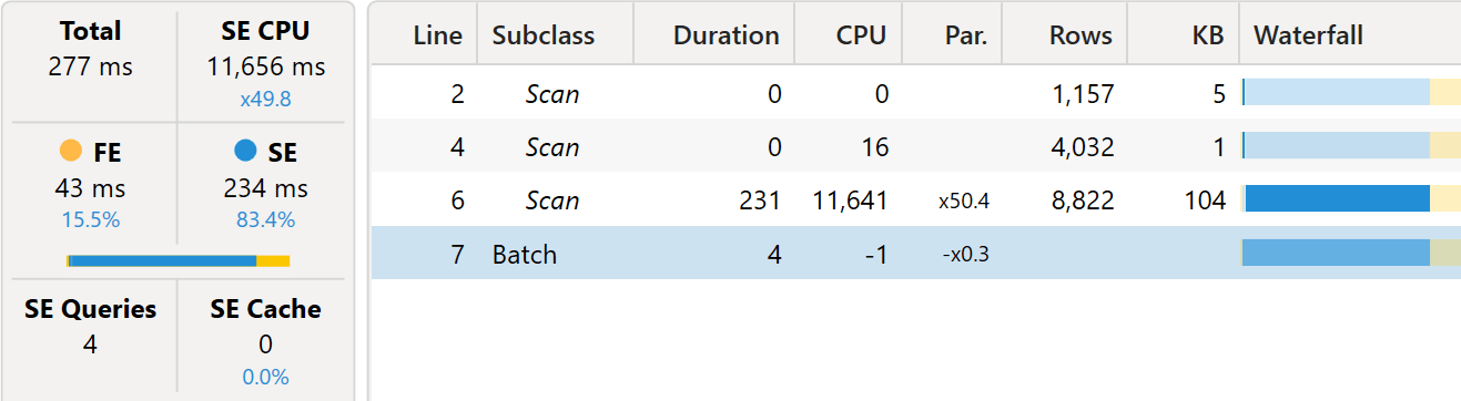
Therefore, the difference that was not noticeable with small datasets becomes an important factor on larger models, where the many-to-many pattern proves to be faster thanks to a better use of the VertiPaq engine.
If instead of using an additive calculation like Sales Amount, we use a distinct count of Sales[CustomerKey], then the behavior of the two models becomes much closer – both on small and large models. First we tested the query with calculation groups and the # Products measure, which computes the distinct count of Sales[ProductKey]:
EVALUATE
    SUMMARIZECOLUMNS (
        'Product'[Brand],
        Customer[Country],
        Customer[Gender],
        Store[Name],
        'Period CG'[Period CG],
        'Period CG'[Ordinal],
        "# Products", [# Products]
    )
The server timings shows a very similar behavior as the additive calculation, the main difference being the calculation that is aggregated.
The same distinct count, when aggregated through the many-to-many pattern, completely changes the query plan by moving to a query plan that is surprisingly close to the one used with the calculation groups.
Despite the number of queries being smaller, the timings are nearly identical. When executed on a larger database, the two queries provide the same results in around the same amount of time.
Conclusions
Creating a table or a calculation group to let users quickly choose time periods is a common requirement in several scenarios. The solution using calculation groups offers a lot of flexibility, with the small disadvantage that developers need to write DAX code for every selection. The many-to-many solution relies on a configuration table that is somewhat less flexible, unless the configuration table becomes more complex and requires more data to define each period.
With small or medium-sized models, the performance of the two solutions is nearly identical. On large models, the solution based on the many-to-many pattern proves to be faster because it relies more heavily on the storage engine. When working with non-additive calculations, both solutions provide the same performance; indeed, the two query plans generated are extremely similar.
If you need to implement this technique in your model, we strongly suggest that you perform a few tests before making your final decision. Always remember that with DAX, data distribution is of paramount importance, and you are very unlikely to share the data distribution of our test models.
Returns the measure that is currently being evaluated.
SELECTEDMEASURE ( )
Returns the dates between two given dates.
DATESBETWEEN ( <Dates>, <StartDate>, <EndDate> )