 Marco Russo
Calculated columns are supported in all the products supporting models for DAX: Power Pivot, Power BI, and Analysis Services Tabular. Calculated tables have been introduced in Analysis Services 2016 and have been available in Power BI since early versions. As of August 2017, Power Pivot does not support calculated tables.
You define both calculated columns and calculated tables using a DAX expression, which the engine evaluates when you refresh one or more partitions or tables of a data model. The engine guarantees that they are evaluated according to any dependencies on other objects in the data model. For example, consider a Product table having a calculated column that computes the sum of the quantity sold by aggregating rows from the Sales table. Every time you refresh the Sales table (or any partition of it), the engine also updates the dependent calculated column in the Product table. Power BI does this automatically, whereas you have a finer control in Analysis Services, where you can rely on the automatic refresh of a Process Full, or control it by using the Process Data and Process Recalc actions.
Similarities between calculated columns and calculated tables end with the dependencies. They are different from a processing point of view, producing different results from a compression storage perspective. A special thanks to Akshai Mirchandani for the clarifications provided to write this article.
Processing of a calculated column
The engine processes a calculated column after it completes the process of the table that the calculated column belongs to. Moreover, when a process operation affects the data of a table referenced by calculated columns in other tables, those calculated columns must be processed too. Thus, when a table process completes, there are several calculated columns that are no longer valid and must be refreshed.
The engine automatically recognizes the order in which the calculated columns must be processed. For each calculated column, the engine iterates the table and evaluates the DAX expression of the calculated column for each row, storing the result in the resulting column structure.
The native columns of a table are processed all at once, and the compression of each column depends on the best sort order of the entire table heuristically found by the engine (if the table is larger than one million rows, this could happen in segments to reduce memory impact). Calculated columns do not participate in the search of the optimal sort order. Thus, the compression of a calculated column cannot take advantage of a different sort order of the table rows.
For these reasons, a calculated column has two disadvantages over native columns:
- It could increase processing time: the evaluation of the DAX expression is sequential, and there could be limits in parallelism of the evaluation of multiple calculated columns.
- It could get a lower compression rate: a native column would participate in the sorting rows process that optimizes the compression rate, whereas a calculated column simply gets the sort order chosen by considering only the native columns of the same table.
If a table has more than one segment, the calculated columns will be split into the same number of segments. After the process, the only difference between a calculated column and a native column is the potential lower efficiency of the compression. However, if there is a one-to-one a correlation between a native column and a calculated column, you might expect no differences at all. For example, if you create a column that denormalizes an attribute key using RELATED or LOOKUPVALUE, the compression of the calculated column will leverage the existing sort order of the native column if the cardinality is the same. If you apply a calculation that changes the cardinality, such as Sales[Quantity] * Sales[Price] or MONTH ( ‘Date'[Date] ), then the new cardinality of the calculated column might not have an optimal sort order for the compression, as it could if it were a native column.
Processing of a calculated table
Like in the case of a calculated column, processing a calculated table happens according to an evaluation order based on the dependencies of the DAX expression used to define the table itself. However, a calculated table includes several columns and all these columns are considered as native columns during the compression. In fact, a calculated table can have additional calculated columns, which are evaluated after the calculated table and follow the same rules described in the previous section.
The steps executed by processing a calculated table are described in the following list:
- The engine parses the DAX expression of the calculated table, building a logical and physical query plan, just like a DAX query (EVALUATE statement).
- An iterator is requested over the physical operator tree.
- This iterator may need to fetch data from Vertipaq, and build intermediate spools – these are not compressed.
- Processing of the data is done over the data returned by the iterator – just like processing over the rows of a table coming from a data source (M query, SQL statement, or anything else).
Step 3 is crucial. If the number of rows produced in the calculated table is very high, there is a good chance the entire table will be materialized in memory (in uncompressed state) before being compressed. This really depends on the query plan and on the query structure. For example, the result of a CROSSJOIN function only materializes the two table expressions used as arguments, whereas an ALL function could materialize all the existing combinations of the columns referenced.
The result of the compression of the calculated table is not different from a regular table read from an external data source or an M query. The engine sorts the rows generated and then compresses all the columns in the same way. All the columns of a calculated table are considered as native columns on this regard.
Compression comparison
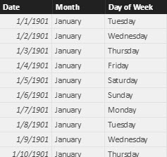
You can observe the differences in storage compression by comparing the results provided by VertiPaq Analyzer using three different techniques to create the same table. In the Power BI example that you can download at the bottom of this article, there are three different versions of the same date table with three columns: Date, Month, and Day of Week. Each table contains all the days for 200 years, from Jan 1, 1901 to Dec 31, 2100.
The columns choice maximizes the visibility of differences and similarities. The use of Date tables is just an example that is easy to reproduce. With other columns for a Date table or different tables you can observe different results, but the principle does not change. Calculated tables and native tables have the same compression, whereas calculated columns might produce different results – often less efficient.
The first table is Date Calc Column: there is a single column Date, generated by an M query that returns only the Date column, and two calculated columns with the following definition:
1 2 | Date[Month] = FORMAT ( [Date], "mmmm" )Date[Day of Week] = FORMAT ( [Date], "dddd" ) |
 Copy
Copy Conventions
The second table is Date Calc Table, produced by a single DAX expression in a calculated table:
1 2 3 4 5 6 7 8 9 | Date Calc Table =ADDCOLUMNS ( CALENDAR ( DATE ( 1901, 1, 1 ), DATE ( 2100, 12, 31 ) ), "Month", FORMAT ( [Date], "mmmm" ), "Day of week", FORMAT ( [Date], "dddd" )) |
The third table is Date M and generates all three columns using an M query.
If you use VertiPaq Analyzer, you will see the results shown in the following picture. Please note you should follow the instructions described in the article Measuring the dictionary size of a column correctly to avoid measuring an inflated dictionary size.
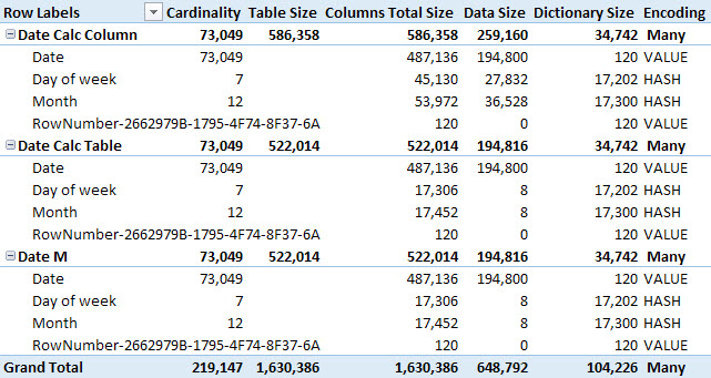
The worst compression is the one obtained by calculated columns, whereas the other two cases (calculated table and M query) have all native columns producing an identical compression. The calculated columns receive rows sorted by date, whereas in the other cases the entire table can be sorted by Month and/or Day of Week columns, obtaining a better compression of these columns that have a low cardinality.
Note: if you are interested in techniques to create calculated tables in DAX, you should also read the article Using GENERATE and ROW instead of ADDCOLUMNS in DAX.
Conclusions
Calculated tables and calculated columns are both generated from DAX expressions evaluated after the process of other tables in a data model. Calculated columns might produce a lower compression rate that could also affect the query performance, requiring more time to scan the column. Calculated tables do not suffer from this issue, even if their content might be completely materialized in memory in uncompressed state before the compression. The memory required to process a calculated table depends on the number of rows and on the query plan of the DAX expression. Usually this is not a real issue for tables that have only tens of thousands of rows or less.
Returns a related value from another table.
RELATED ( <ColumnName> )
Retrieves a value from a table.
LOOKUPVALUE ( <Result_ColumnName>, <Search_ColumnName>, <Search_Value> [, <Search_ColumnName>, <Search_Value> [, … ] ] [, <Alternate_Result>] )
Returns a number from 1 (January) to 12 (December) representing the month.
MONTH ( <Date> )
Returns a table that is a crossjoin of the specified tables.
CROSSJOIN ( <Table> [, <Table> [, … ] ] )
Returns all the rows in a table, or all the values in a column, ignoring any filters that might have been applied.
ALL ( [<TableNameOrColumnName>] [, <ColumnName> [, <ColumnName> [, … ] ] ] )