 Alberto Ferrari
If you are a loyal reader of this website, you probably already know that, in DAX, evaluation contexts are everything. We oftentimes teach to our students that once they understand evaluation contexts, DAX will hide no secret to them.
Yet, even with a solid understanding of evaluation contexts, it is still very easy to fall in some traps and, in this article, you will learn the subtle difference between using ALLEXCEPT or ALL and VALUES as filter parameters of CALCULATE.
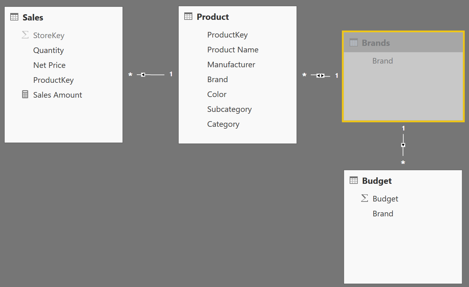
In order to elaborate on this topic, we use a scenario that happens somewhat frequently, when you need to join two fact table with a dimension but at a different granularity. We discussed these kind of data models in this article but, with Power BI and Analysis Services 2016 (SSAS 2016), the presence of bidirectional filtering lets you use a different (and better) pattern. The data model used for this demo is the following one:
Since its behavior is not trivial, it is worth spending a few words describing it, because this is a pattern you are likely to encounter several times, whenever you need to use dimensions with different granularities.
The budget table contains data at the Brand granularity. The Product dimension contains the Brand column but it has a higher granularity, which is the granularity of the individual product. This is needed because Sales relate to a product, not only to a brand. Thus, you need to relate Budget with Product, but with a different granularity.
If you use SSAS 2012/2014 (or any version of Power Pivot in Excel), a good option is to change the model by building an intermediate dimension (Brands, in this case) that is linked to both Product and Budget. A filter on Brands will reach Product (and, in turn, Sales) and Budget at the same time. It is a good practice hiding the Brand column from Product, so that the user will use only Brands to filter the brands. If he filters the Brand column in Product, such a filter will never be able to reach Budget.
In Power BI and SSAS 2016 you have a better option. By setting the relationship between Product and Brands as a bidirectional one (as we did in the model shown), you obtain the effect that a filter on Product will filter Brands, because of the bidirectional filtering, and, from there, it will reach Budget. This is very convenient because, with Power BI and SSAS 2016, you can let the user filter Store and keep the Brands table hidden. At the end, Brands is only a technical table useful to propagate a filter, but it is not a real business entity that you want to show to your users.
Besides, there is an interesting optimization that the DAX engine carries on: If you do not filter the Product table, then your calculations will not use the intermediate Brands table as a filter, obtaining in this way better performances if the table does not need to be traversed. Without bidirectional filters, DAX does not take advantage of this optimization and can result in worse performance.
After this small digression, which is probably worth an article by itself, let us speak about DAX. The model shown works fine, as long as you browse data at the Brand granularity. You can see that in the following report.
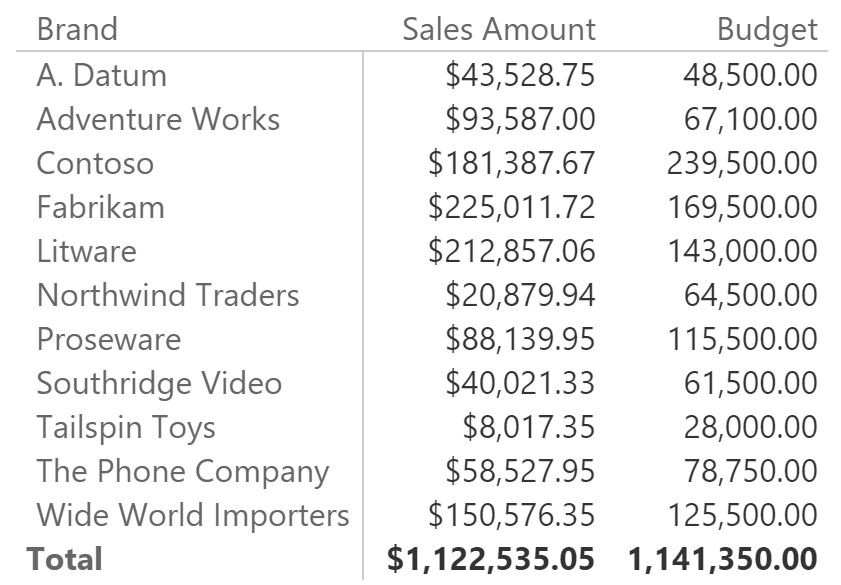
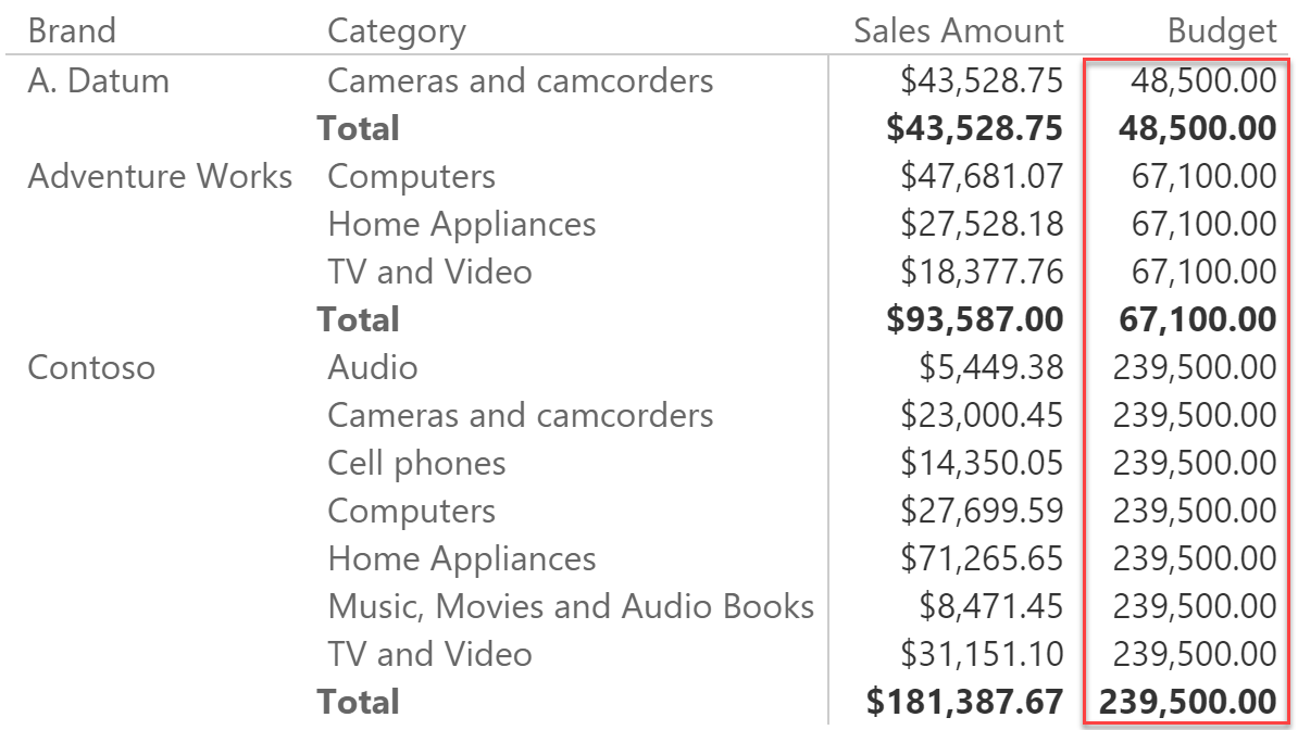
Things are a bit more complex if you browse data at a higher granularity because, if you slice by category too, the budget is repeated with the same values for all the categories. In fact, the filter on the category is not active against the budget, because the budget exists only at the brand level, not at the brand/category one.
The solution is to check the granularity by counting the number of products at the two different granularities in order to detect which level of detail the user is browsing. This can be accomplished by creating two measures:
NumOfProducts := COUNTROWS ( 'Product' )

NumProducts at Brand Granularity :=
CALCULATE (
    [NumOfProducts],
    ALLEXCEPT ( 'Product', 'Product'[Brand] )
)
You can see that the two measures, projected on a report, show different values only when you are browsing data at a higher granularity:
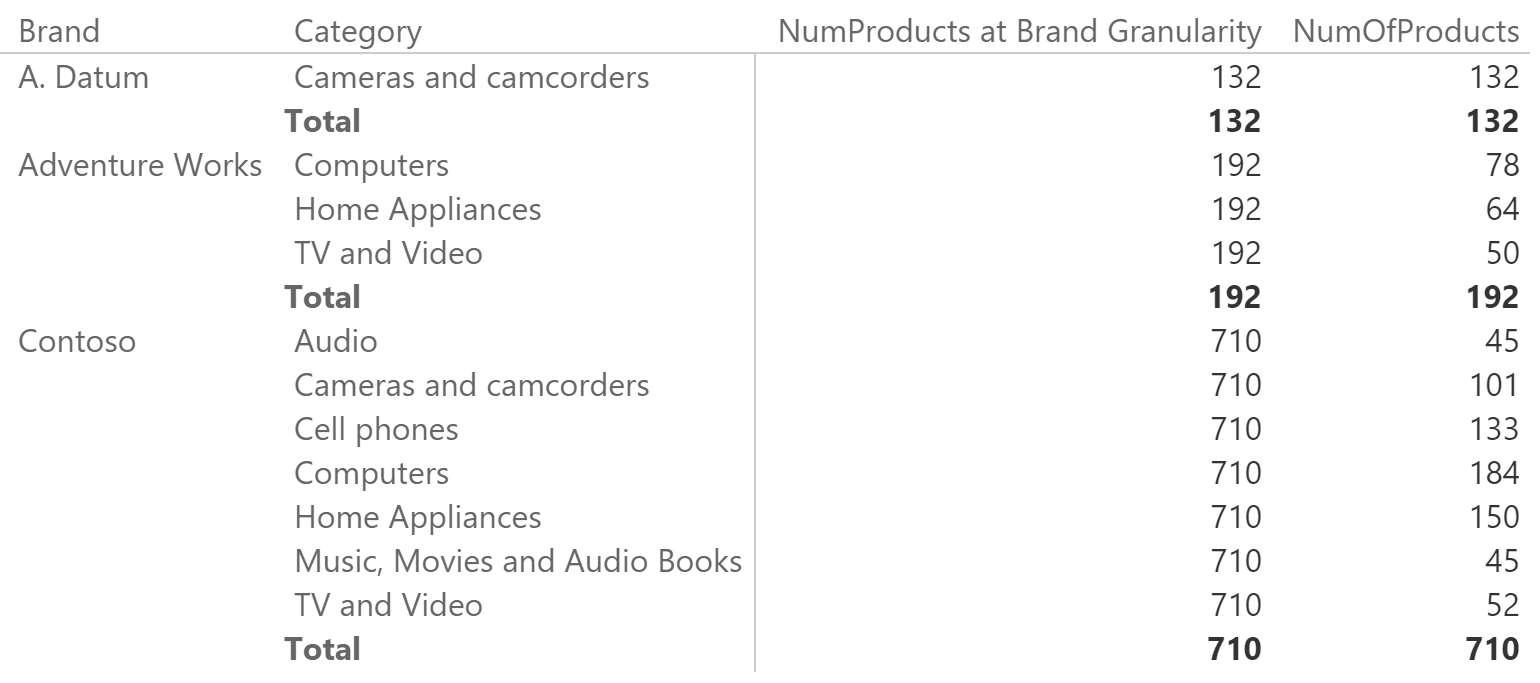
As a method to check when you go at a higher granularity, this technique looks fine, and you can use a simple IF statement to visualize the budget only when the granularity is the right one.
Budget Value :=
IF (
    [NumOfProducts] = [NumProducts at Brand Granularity],
    SUM ( Budget[Budget] )
)
However, if you browse the values at a lower granularity, things start to be more complex. To demonstrate this, we added a column to the Product table that contains “Internal” for only the two brands A.Datum and Contoso. This new column has a lower granularity than that of the Brand, so you would expect to be able to slice the budget at that level. Unfortunately, the result is the following:
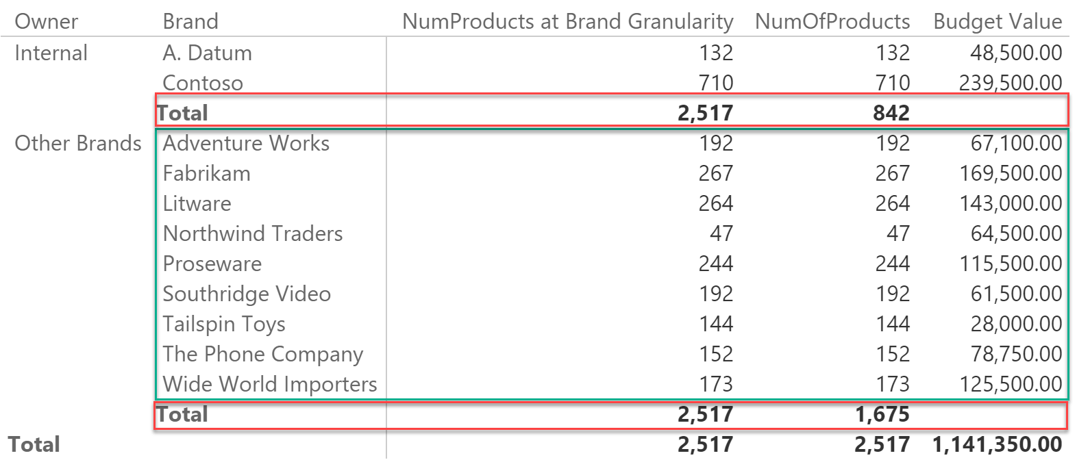
Why is that you can show the budget at the Brand level but not at a lower granularity? The subtotals are missing. The problem is in the code that computes the number of products at the brand granularity, because it uses the ALLEXCEPT function.
NumProducts at Brand Granularity :=
CALCULATE (
    [NumOfProducts],
    ALLEXCEPT ( 'Product', 'Product'[Brand] )
)
ALLEXCEPT removes any filter from a table apart from the columns that you are explicit about, using them as parameters. In the example code, ALLEXCEPT removes any filter from the Product table apart from the one on the Brand column. When Brand is part of the filter context, as it happens for all the rows in the green box, the formula computes the correct value. But in the red boxes, the filter context contains only the Owner column, and Brand is not part of it. Yes, whenever the owner is Internal you see only two brands, but this is not an effect of a direct filter on the brand column, it is a cross-filter coming from the owner column. Let us repeat this important concept: there is no filter on brand, there is only a filter on the owner. The fact that – in the report – you see only two brands is a side effect of the filter on the owner.
Thus, when you remove the filter from all the columns, apart from the Brand, you are removing – in fact – all the filters from the table, and this is the reason why you see – as the number of products – the grand total of all products.
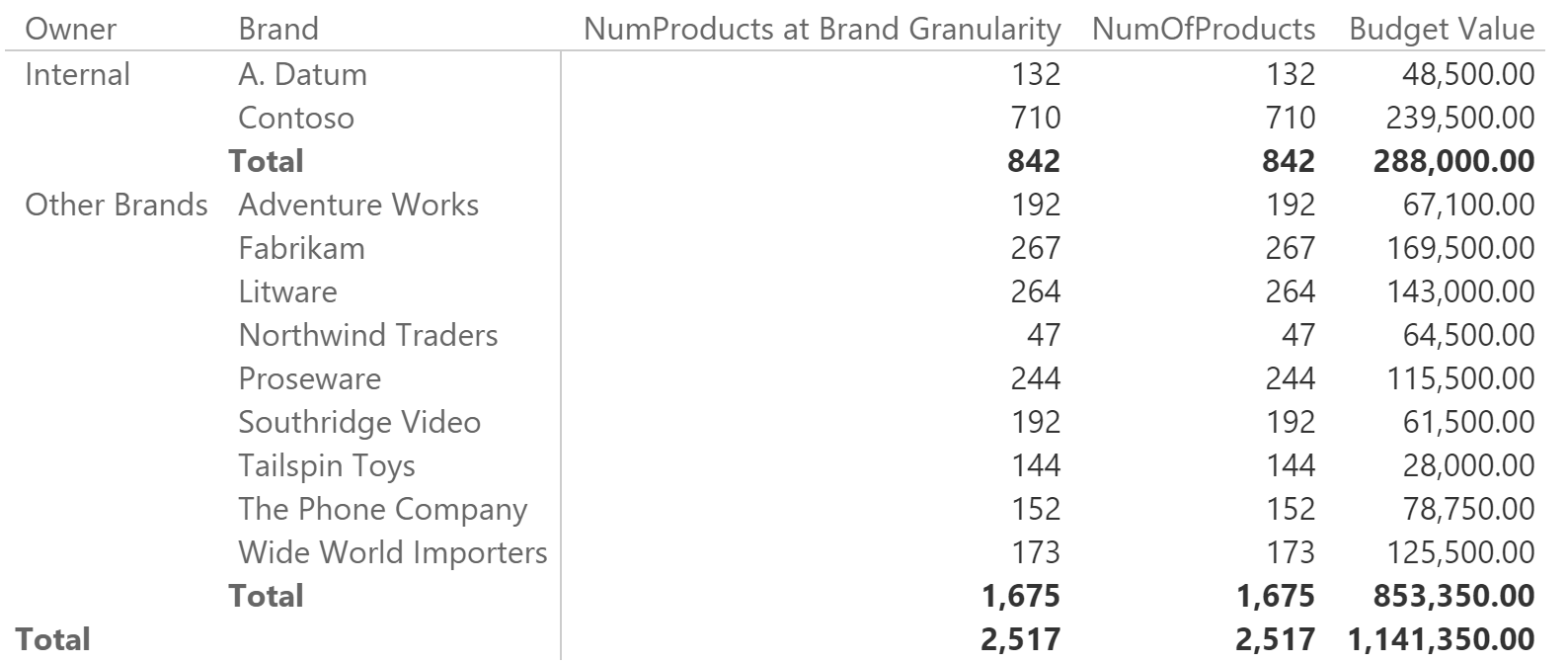
There are two ways of avoiding this problem: either you list, in the ALLEXCEPT function, all the columns at any granularity which is lower than the budget one (in this case, the only column would be Owner), or you replace ALLEXCEPT with a pair of ALL and VALUES. The two following measures will work:
NumProducts at Brand Granularity :=
CALCULATE (
    [NumOfProducts],
    ALLEXCEPT( 'Product', 'Product'[Brand], 'Product'[Owner] )
)

NumProducts at Brand Granularity :=
CALCULATE (
    [NumOfProducts],
    ALL ( 'Product' ),
    VALUES ( 'Product'[Brand] )
)
As you can see, using this measure the result is the expected one:
Are there any differences between the two versions? Yes, but they are somewhat hard to notice. The version with ALLEXCEPT gives to the engine a better indication of what you want to retrieve. By analyzing the query plan, you will see that the DAX engine performs fewer scans and results in slightly better performance. The version with ALL and VALUES cannot be optimized at its best, because the code is harder to read, even for the optimizer, resulting in a slightly more work on the Formula Engine side. The version with ALLEXCEPT is faster but, because the Product table is a tiny one, the difference in terms of speed is hard to notice. With larger tables and/or more complex code, you might experience different results.
Although a bit faster, the version with ALLEXCEPT requires you to hardcode – in a measure – the structure of the granularity of your tables and requires more maintenance over time (basically, whenever you add a column to the model that has a granularity lower than that of the brand). It is very likely that you will forget to update the measure, sooner or later.
Our personal choice is to go for the ALL and VALUES version, and rely on the ALLEXCEPT one only if we are seeking for top performance. Nevertheless, performance is only an aspect of the whole story. Sometimes, as in this example, different versions of the same code look to return the very same value, but only because the difference is hard to spot. There is a big semantic difference between using ALLEXCEPT versus ALL and VALUES together. The former removes filters, the latter removes and restores filters by taking into account the previous cross-filtering, which is ignored by ALLEXCEPT.
These small details make a real difference between a formula that always works and one that sometimes works, but other times returns a wrong result. This is why learning all the secrets of evaluation contexts is time well-spent.
Returns all the rows in a table except for those rows that are affected by the specified column filters.
ALLEXCEPT ( <TableName>, <ColumnName> [, <ColumnName> [, … ] ] )
Returns all the rows in a table, or all the values in a column, ignoring any filters that might have been applied.
ALL ( [<TableNameOrColumnName>] [, <ColumnName> [, <ColumnName> [, … ] ] ] )
When a column name is given, returns a single-column table of unique values. When a table name is given, returns a table with the same columns and all the rows of the table (including duplicates) with the additional blank row caused by an invalid relationship if present.
VALUES ( <TableNameOrColumnName> )
Evaluates an expression in a context modified by filters.
CALCULATE ( <Expression> [, <Filter> [, <Filter> [, … ] ] ] )
Checks whether a condition is met, and returns one value if TRUE, and another value if FALSE.
IF ( <LogicalTest>, <ResultIfTrue> [, <ResultIfFalse>] )