 Marco Russo & Alberto Ferrari
Our readers know SQLBI’s position on bidirectional relationships: they are a powerful tool that should be used with great care or avoided altogether in most scenarios. There actually is one scenario where bidirectional relationships are useful: when you need to create a model involving a many-to-many relationship between dimensions. In this scenario, using a bidirectional filter relationship is the suggested solution. Nonetheless, one of the reasons a bidirectional relationship cannot be created may be ambiguity.. If you are facing this situation, you can use a different modeling technique based on a limited many-to-many cardinality relationship, which would work even when it is set as a unidirectional relationship. The choice between the two models is not easy to make. Both come with advantages and disadvantages that need to be understood in depth in order to make the right decision.
In this article, we first provide a description of the two techniques, and then we proceed with the performance analysis of both solutions, to provide insights on which technique to use and when.
The scenario
In the Contoso database, there are no many-to-many relationships. Therefore, we created a many-to-many relationship between the Customer and the Sport tables. We assigned to each customer a certain number of sports that they play. Because each customer may play multiple sports, and each sport may be played by multiple customers, the natural relationship between customers and sports is a many-to-many relationship.
The canonical way to model this relationship is shown below.

A filter from Sport flows to CustomerSport, then it goes through the bidirectional relationship to Customer to finally reach Sales. By using this model, you can slice Sales by Sport thus obtaining the usual many-to-many non-additive behavior. This is the way we have been teaching many-to-many relationships over the years.
We have recently been discussing another possible option to model this scenario by using limited many-to-many cardinality relationships.
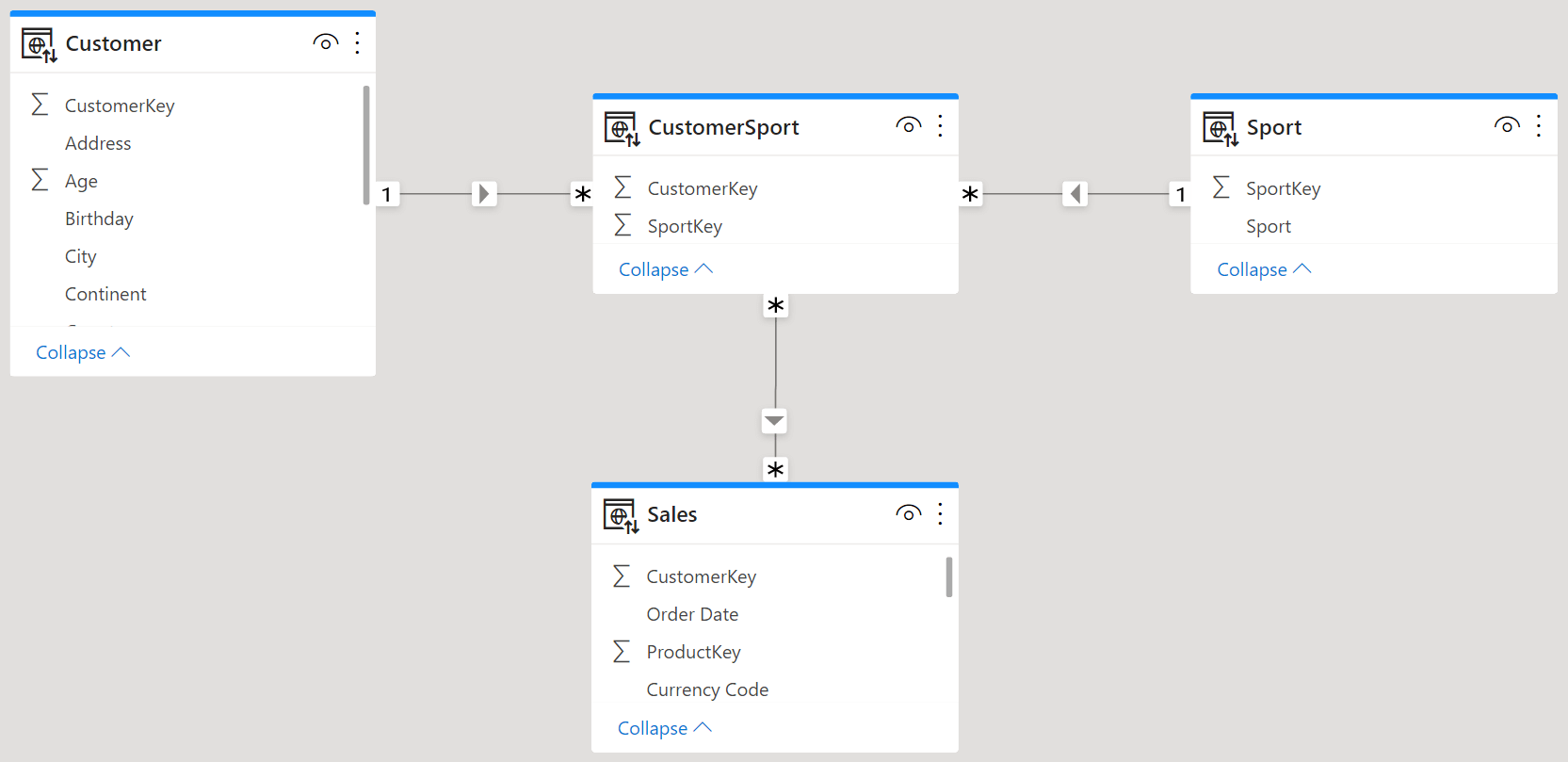
This second model is visually more appealing and it does not require bidirectional relationships – which is most relevant. A filter from either Customer or Sport is applied first to CustomerSport and is then moved to Sales through the many-to-many cross-filter relationship.
Because of the absence of bidirectional relationships in this model, the model is surely more flexible than the previous one. That said, is it also better or at least comparable in terms of performance? Unfortunately, the quick answer is “it depends”. This second model produces different query plans that can be better in some scenarios, and not as good in other scenarios. It all depends on the tables involved in the specific query. Therefore, the new model is an option that should be tested thoroughly before you move it into production.
In order to prove the above statement, we obviously need to perform tests. Before going into the details of the tests, we look at a few considerations. In order to distinguish between the two models, we call the first one the “canonical” model, whereas the second model presented is the “new” model.
The weak point of canonical many-to-many relationships is the bidirectional relationships. It is a weak point from the modeling point of view, because it might introduce ambiguity. It is also a weak point from the performance point of view, because transferring a filter from the many-side to the one-side is always more expensive than doing the opposite.
The new solution does not have bidirectional relationships, but it also presents two weak points. First, the relationship between CustomerSport and Sales is a limited relationship. Performance-wise, limited relationships are slow because they are not materialized. What we should measure is whether a bidirectional relationship is slower than a many-to-many cardinality relationship or not. But then there is another issue. In the canonical model, Customer is linked directly to Sales through a regular 1:M relationship. In the new model, Customer is linked to Sales only through the bridge table. This means that the engine traverses the many-to-many relationship whenever a user slices by attributes of Customer or Sport. In the canonical model, if a user browses by customer, then the bridge table is not part of the game. In the new model, the bridge table always plays an important role. In the new model, a user browsing by customer runs a query that always uses CustomerSport to filter Sales. This important detail is the weakest point of the new model, as we will analyze further with the queries.
Testing performance
The considerations so far are useful to define the tests to perform. We will check the performance of computing Sales Amount (a measure that scans the Sales table) filtering by Sport and by Customer in both scenarios. The model we are using is a Contoso version with 1.4 billion rows. The CustomerSport table contains around 3 million rows: we created a model where each customer plays between zero sport and three different sports.
The first query groups by Sport[Sport] and it computes Sales Amount. In its simplicity, the query needs to traverse the CustomerSport relationship and use only the Sport table to group by:
1 2 3 4 5 | EVALUATESUMMARIZECOLUMNS ( Sport[Sport], "Amt", [Sales Amount]) |
 Copy
Copy Conventions
In order to deepen our knowledge of how many-to-many relationships are evaluated, we also analyze a second, slightly more complex query, that groups by both Sport and Customer:
1 2 3 4 5 6 | EVALUATESUMMARIZECOLUMNS ( Customer[Continent], Sport[Sport], "Amt", [Sales Amount]) |
Finally, in the last query we analyze groups by Customer only. In the canonical model, this query does not need to traverse the CustomerSport table. In the new model, on the other hand, this query needs to use CustomerSport anyway, because of the way relationships are laid out:
1 2 3 4 5 | EVALUATESUMMARIZECOLUMNS ( Customer[Continent], "Amt", [Sales Amount]) |
Tests on the canonical model
First, this is the canonical model, with one bidirectional relationship between Customer and CustomerSport.
Let us now run the queries on the canonical model. The first query groups by Sport:
1 2 3 4 5 | EVALUATESUMMARIZECOLUMNS ( Sport[Sport], "Amt", [Sales Amount]) |
First, the execution time. The query uses 385,984 milliseconds of storage engine CPU, with a tiny amount of formula engine (10 milliseconds).

The query plan is interesting to analyze. The entire calculation is pushed down to the storage engine, with the aid of temporary tables. Here are the details:
1 2 3 4 5 6 7 8 9 10 11 12 13 14 15 16 17 18 19 20 21 22 23 24 25 26 27 28 29 30 31 32 33 34 35 36 37 38 39 40 41 42 43 44 45 46 47 | ---- First we retrieve the pairs of CustomerKey and Sport from CustomerSport--DEFINE TABLE '$TTable3' := SELECT 'Customer'[CustomerKey], 'Sport'[Sport]FROM 'CustomerSport' LEFT OUTER JOIN 'Customer' ON 'CustomerSport'[CustomerKey]='Customer'[CustomerKey] LEFT OUTER JOIN 'Sport' ON 'CustomerSport'[SportKey]='Sport'[SportKey];---- Here we extract the CustomerKey values in a bitmap--DEFINE TABLE '$TTable4' := SELECTSIMPLEINDEXN ( '$TTable3'[Customer$CustomerKey] )FROM '$TTable3';---- Here is where the actual computation happens. -- Note that the first INNER JOIN is with Table3, to retrieve the Sport-- Table4 is used to further filter the scanning of Sales--DEFINE TABLE '$TTable1' := SELECT '$TTable3'[Sport$Sport], SUM ( '$TTable2'[$Measure0] )FROM '$TTable2' INNER JOIN '$TTable3' ON '$TTable2'[Customer$CustomerKey]='$TTable3'[Customer$CustomerKey] REDUCED BY '$TTable2' := WITH $Expr0 := 'Sales'[Quantity] * 'Sales'[Net Price] SELECT 'Customer'[CustomerKey], SUM ( @$Expr0 ) FROM 'Sales' LEFT OUTER JOIN 'Customer' ON 'Sales'[CustomerKey]='Customer'[CustomerKey] WHERE 'Customer'[CustomerKey] ININDEX '$TTable4'[$SemijoinProjection]; |
The engine performs its calculation in three steps, corresponding to the three storage engine queries:
- First it retrieves the pairs of SportKey and CustomerKey from CustomerSport.
- Next, it generates a bitmap containing the CustomerKey values present in CustomerSport. This table is going to be used in the next step, to filter the customers being scanned from Sales. Indeed, because we are only interested in slicing by sport, customers not playing any sport will be ignored.
- The last step is where the actual calculation happens. The engine scans Sales and retrieves only the customers that are in CustomerSport (Table2). It joins this result with Table3, that maps customers to sports.
Despite being a complex plan, you see that the entire calculation has been pushed down to the storage engine. Nonetheless, the storage engine cannot handle bidirectional filters by itself, therefore it needs to prepare these temporary tables to produce the correct joins.
The overall logic is also visible in the physical query plan. Indeed, the physical query plan is made of only four lines that retrieve the 45 rows corresponding to the sport, entirely computed by the storage engine.

Because the entire calculation is pushed down to the storage engine, the degree of parallelism used is very good: it shows x49.7 on a machine with 64 virtual cores, as a further demonstration that the engine is maximizing its use of CPU power.
We described the plan in so much detail because it is important to be able to compare this first plan with the following plans. There are significant differences in the performance of different queries on different models and details matter.
Let us now add Customer[Continent] to the query. From a DAX point of view, the difference is not that complex: just one more line in the SUMMARIZECOLUMNS groupby list:
1 2 3 4 5 6 | EVALUATESUMMARIZECOLUMNS ( Customer[Continent], Sport[Sport], "Amt", [Sales Amount]) |
Despite being very close to the previous query, the timings are now very different.

Before diving into the details, please note that the degree of parallelism is largely reduced: it now shows x23.5, less than half what we had in the previous query. Moreover, the formula engine time has greatly increased: it went from 10 to 3,120 milliseconds.
In order to understand the reasons why we have this performance degradation, we need to dive deeper. These are the storage engine queries:
1 2 3 4 5 6 7 8 9 10 11 12 13 14 15 16 17 18 19 20 21 22 23 24 25 26 27 28 29 30 | ---- Here we retrieve the Sales Amount for each customer, without reducing the -- set to only the customers being filtered by the CustomerSport table, as it-- happened in the previous query--WITH $Expr0 := 'Sales'[Quantity] * 'Sales'[Net Price] SELECT 'Customer'[CustomerKey], 'Customer'[Continent], SUM ( @$Expr0 )FROM 'Sales' LEFT OUTER JOIN 'Customer' ON 'Sales'[CustomerKey]='Customer'[CustomerKey];---- Here we match CustomerKey values with Customer[Continent] and Sport-- by scanning Customersport, Customer and Sport together--SELECT 'Customer'[CustomerKey], 'Customer'[Continent], 'Sport'[Sport]FROM 'CustomerSport' LEFT OUTER JOIN 'Customer' ON 'CustomerSport'[CustomerKey]='Customer'[CustomerKey] LEFT OUTER JOIN 'Sport' ON 'CustomerSport'[SportKey]='Sport'[SportKey]; |
This time, the storage engine does not actually compute the values being returned by the query. It first retrieves the sales amount for each customer key, and then another table that maps customer keys with continent and sport.
The absence of further calculations in the storage engine is a clear indication that the real many-to-many computation happens in the formula engine. Hence the large increase in formula engine use. Moreover, because it will be the formula engine that computes the actual values, this means that the data structures containing the partial values need to be passed back to the formula engine. This is the biggest difference between the two query plans: the previous query plan performed all its computation inside the storage engine, whereas this latter query plan requires moving large amounts of data back to the formula engine.
You can appreciate this “detail” by looking at the physical query plan, that now clearly indicates that the table with Continent and Sport (135 rows) is joined with the larger table containing Sales Amount by CustomerKey (2,802,660 rows) in the formula engine.

Because it involves the formula engine, this query plan is clearly suboptimal compared to the previous query plan.
Things are very different when the CustomerSport table is not part of the game. Indeed, the last query we analyze slices the sales amount only by Customer[Continent]. Because of the way we laid out relationships, there is no need to use the CustomerSport table, because Customer can apply its filtering directly to Sales:
1 2 3 4 5 | EVALUATESUMMARIZECOLUMNS ( Customer[Continent], "Amt", [Sales Amount]) |
The server timings are excellent.

There is no formula engine involved, the degree of parallelism is an awesome x54.5 and the entire query is executed using only 16,609 milliseconds of storage engine CPU. This is the behavior that can be expected of DAX with regular one-to-many relationships. The entire calculation is performed by its best engine: the storage engine.
Now that we have executed and analyzed the three queries, we can draw conclusions about the canonical model. When the query involves only the Sport table and the calculation can be pushed down to the storage engine, Tabular generates a very good query plan that uses the storage engine at its best. The query is heavy, but by using temporary tables that are not moved out of VertiPaq, the degree of parallelism is good. When the query becomes more complex, the formula engine is required – which greatly slows down the entire query. If the engine does not use the CustomerSport bridge table, then VertiPaq performs at its best: no formula engine is involved and the query does not even need temporary structures.
Tests on the new model
Now that we have a good understanding of the way many-to-many relationships are resolved in the canonical model, we can perform the same three tests on the new model to check how it behaves. This below is what the new model looks like.
There are no bidirectional relationships. This time, Customer is linked to Sales through CustomerSport, the same way Sport is.
We start with the first query, that groups by Sport only:
1 2 3 4 5 | EVALUATESUMMARIZECOLUMNS ( Sport[Sport], "Amt", [Sales Amount]) |
First, the timings:

The entire query is resolved in the storage engine. There are a few queries running on a single core, and the main query achieves a very good degree of parallelism. Overall, the total timing is very close to what we achieve with the canonical model.
Because the layout of the relationships is different, the query plan is also slightly different from the one obtained with the canonical model – although the overall logic is very close. Let us look at the storage engine queries:
1 2 3 4 5 6 7 8 9 10 11 12 13 14 15 16 17 18 19 20 21 22 23 24 25 26 27 28 29 30 31 32 33 34 35 36 37 38 39 40 41 42 43 44 45 46 47 48 49 50 51 52 53 54 | ---- Here we retrieve Sport and CustomerKey scanning CustomerSport--DEFINE TABLE '$TTable3' := SELECT 'Sport'[Sport], 'CustomerSport'[CustomerKey]FROM 'CustomerSport' LEFT OUTER JOIN 'Sport' ON 'CustomerSport'[SportKey]='Sport'[SportKey];---- Here we retrieve CustomerKey only from Table3, which is derived from CustomerSport--DEFINE TABLE '$TTable4' := SELECT '$TTable3'[CustomerSport$CustomerKey]FROM '$TTable3';---- Table5 contains the values of CustomerKey that are present in Sales, it will-- be used later to reduce the scanning of Sales--DEFINE TABLE '$TTable5' := SELECT RJOIN ( '$TTable4'[CustomerSport$CustomerKey] )FROM '$TTable4' REVERSE BITMAP JOIN 'Sales' ON '$TTable4'[CustomerSport$CustomerKey]='Sales'[CustomerKey];---- In this final query, Table5 is used to reduce the scanning of Sales to retrieve-- the final result--DEFINE TABLE '$TTable1' := SELECT '$TTable3'[Sport$Sport], SUM ( '$TTable2'[$Measure0] )FROM '$TTable2' INNER JOIN '$TTable3' ON '$TTable2'[Sales$CustomerKey]='$TTable3'[CustomerSport$CustomerKey] REDUCED BY '$TTable2' := WITH $Expr0 := 'Sales'[Quantity] * 'Sales'[Net Price] SELECT 'Sales'[CustomerKey], SUM ( @$Expr0 ) FROM 'Sales' WHERE 'Sales'[CustomerKey] ININDEX '$TTable5'[$SemijoinProjection]; |
As you see, despite the number of storage engine queries being different, the overall logic is the same as with the canonical model. The physical query plan is the final demonstration that the plans are actually nearly identical and that the entire work is performed in the storage engine.

Time to look at the second query, involving both Customer and Sport:
Time to look at the second query, involving both Customer and Sport:
1 2 3 4 5 6 | EVALUATESUMMARIZECOLUMNS ( Customer[Continent], Sport[Sport], "Amt", [Sales Amount]) |
Here we can appreciate the first important difference between the canonical model and the new model. In this scenario, the canonical model involved heavy usage of the formula engine because it did not rely on the approach used in the previous query. Indeed, the shape of the relationships between Customer and Sales was not the same as the shape of the relationships between Sport and Customer.
In the new model, Customer and Sport are related to CustomerSport using the very same type of relationship. Consequently, the timings and the format of the internal queries are close to the ones observed in the previous model.

The considerations for this query are the same as for the previous model. There is nearly no formula engine used: the entire query is being executed in the storage engine. This is different from the same query on the canonical model.
In the canonical model, adding Customer triggered a severe degradation of performance, with higher use of the formula engine. In the new model, adding more filters is not an issue. Regarding this, the new model performs significantly better. Let us look at the details of the storage engine queries, to obtain a better picture:
1 2 3 4 5 6 7 8 9 10 11 12 13 14 15 16 17 18 19 20 21 22 23 24 25 26 27 28 29 30 31 32 33 34 35 36 37 38 39 40 41 42 43 44 45 46 47 48 49 50 51 52 53 54 55 56 57 | ---- Here we retrieve Sport, Continent, and CustomerKey scanning CustomerSport--DEFINE TABLE '$TTable3' := SELECT 'Customer'[Continent], 'Sport'[Sport], 'CustomerSport'[CustomerKey]FROM 'CustomerSport' LEFT OUTER JOIN 'Customer' ON 'CustomerSport'[CustomerKey]='Customer'[CustomerKey] LEFT OUTER JOIN 'Sport' ON 'CustomerSport'[SportKey]='Sport'[SportKey];---- Here we retrieve CustomerKey only from Table3, which is derived from CustomerSport--DEFINE TABLE '$TTable4' := SELECT '$TTable3'[CustomerSport$CustomerKey]FROM '$TTable3';---- Table5 contains the values of CustomerKey that are present in Sales, it will-- be used later to reduce the scanning of Sales--DEFINE TABLE '$TTable5' := SELECTRJOIN ( '$TTable4'[CustomerSport$CustomerKey] )FROM '$TTable4' REVERSE BITMAP JOIN 'Sales' ON '$TTable4'[CustomerSport$CustomerKey]='Sales'[CustomerKey];---- In this final query, Table5 is used to reduce the scanning of Sales to retrieve-- the final result--DEFINE TABLE '$TTable1' := SELECT '$TTable3'[Customer$Continent], '$TTable3'[Sport$Sport], SUM ( '$TTable2'[$Measure0] )FROM '$TTable2' INNER JOIN '$TTable3' ON '$TTable2'[Sales$CustomerKey]='$TTable3'[CustomerSport$CustomerKey] REDUCED BY '$TTable2' := WITH $Expr0 := 'Sales'[Quantity] * 'Sales'[Net Price] SELECT 'Sales'[CustomerKey], SUM ( @$Expr0 ) FROM 'Sales' WHERE 'Sales'[CustomerKey] ININDEX '$TTable5'[$SemijoinProjection]; |
As you see, apart from a few differences in the columns being used in the query, the overall structure is identical to the structure in the previous model. The query plan is – again – identical.

In this second query, the new model performs better than the canonical model. This is already extremely interesting because it shows that depending on the kind of queries that you plan to execute on a model, one model performs better than the other.
Unfortunately, the new model falls short on the third query – the query that uses a filter on Customer to reach Sales. In the canonical model, the relationship between Customer and Sales is direct. Therefore, the entire query is executed using a single xmSQL query that performs great:
1 2 3 4 5 | EVALUATESUMMARIZECOLUMNS ( Customer[Continent], "Amt", [Sales Amount]) |
In the new model, the engine needs to still use CustomerSport to reach Sales. Therefore, the third query runs at nearly the same speed as the previous two and the benefit is lost. Here are the timings in the picture below.

Because Continent contains slightly fewer values, and not all the customers play all the sports, the data structures used by the query are slightly smaller and the execution time is slightly shorter. Overall, the format of the storage engine queries is identical to the previous two, and not worth repeating a third time.
In this third scenario, the performance of the model is much poorer than the performance of the canonical model. Again, this is an interesting result as it shows that you need to make choices based on the kinds of queries being executed. If you mostly do not use the many-to-many relationship between Customer and Sport and you rely more on the direct relationship between Customer and Sales for most of your calculations, then the canonical model performs better. On the other hand, if the many-to-many structure is always part of the queries, then the new model comes with interesting advantages.
Optimizing the new model
Based on an interesting comment from Daniel Otykier, we updated this article with further content. We also recorded an unplugged video while analyzing the performance of the suggested changes. Indeed, Daniel noted that the relationships in the new model can be modified to obtain the best of both worlds. Instead of linking Customer to CustomerSport, we link Customer directly to Sales.

In this scenario, both CustomerSport and Customer are linked to Sales using the CustomerKey column. Therefore, the same Sales[CustomerKey] column is being filtered directly by Customer and indirectly by Sport, through CustomerSport.
This model does not contain bidirectional relationships, therefore it does not suffer from the performance penalty of the canonical model; it shows a direct relationship between Customer and Sales, therefore providing optimal performance when Customer filters Sales. On the other hand, the model is missing the relationship between Customer and Sport, because the bridge table no longer links the two dimensions. CustomerSport now links only Sport to Sales. Therefore, determining the sports played by customers is more complex in this model.
We start with the first query, that groups by Sport only:
1 2 3 4 5 | EVALUATESUMMARIZECOLUMNS ( Sport[Sport], "Amt", [Sales Amount]) |
Performance and query plan are identical to the new model, because the only tables involved are Sport, CustomerSport, and Sales.

We do not provide here the detailed xmSQL queries, because they are identical to the ones shown for the new model. Instead, it is interesting to see the behavior of this optimized version when Customer is involved in the query:
1 2 3 4 5 6 | EVALUATESUMMARIZECOLUMNS ( Customer[Continent], Sport[Sport], "Amt", [Sales Amount]) |
Now the filtering happens with two different paths. Sport filters Sales through the bridge table, whereas Customer filters Sales directly. Both filters are working on the same Sales[CustomerKey] column.

The xmSQL code executed is rather interesting. This time, the join between Customer and Sales happens in the table used to reduce the join. Indeed, the Customer[Continent] is gathered only during the last xmSQL query:
1 2 3 4 5 6 7 8 9 10 11 12 13 14 15 16 17 18 19 20 21 22 23 24 25 26 27 28 29 30 31 32 33 34 35 36 37 38 39 40 41 42 43 44 45 46 47 48 49 50 51 52 53 54 55 56 57 58 59 | ---- Here we retrienve Sport and CustomerKey by scanning CustomerSport--DEFINE TABLE '$TTable3' := SELECT 'Sport'[Sport], 'CustomerSport'[CustomerKey]FROM 'CustomerSport' LEFT OUTER JOIN 'Sport' ON 'CustomerSport'[SportKey]='Sport'[SportKey] ---- Here we retrieve CustomerKey only from Table3, which is derived from CustomerSport--DEFINE TABLE '$TTable4' := SELECT '$TTable3'[CustomerSport$CustomerKey]FROM '$TTable3' ---- Table5 contains the values of CustomerKey that are present in Sales; it will-- be used later to reduce the scanning of Sales--DEFINE TABLE '$TTable5' := SELECT RJOIN ( '$TTable4'[CustomerSport$CustomerKey] ) FROM '$TTable4' REVERSE BITMAP JOIN 'Sales' ON '$TTable4'[CustomerSport$CustomerKey]='Sales'[CustomerKey] ---- In this final query, Table5 is used to reduce the scanning of Sales to retrieve-- the final result--DEFINE TABLE '$TTable1' := SELECT '$TTable2'[Customer$Continent], '$TTable3'[Sport$Sport], SUM ( '$TTable2'[$Measure0] )FROM '$TTable2' INNER JOIN '$TTable3' ON '$TTable2'[Sales$CustomerKey]='$TTable3'[CustomerSport$CustomerKey] REDUCED BY '$TTable2' := WITH $Expr0 := 'Sales'[Quantity] * 'Sales'[Net Price] SELECT 'Customer'[Continent], 'Sales'[CustomerKey], SUM ( @$Expr0 ) FROM 'Sales' LEFT OUTER JOIN 'Customer' ON 'Sales'[CustomerKey]='Customer'[CustomerKey] WHERE 'Sales'[CustomerKey] ININDEX '$TTable5'[$SemijoinProjection]; |
There is a slight degradation in performance. Yet the degradation is much lower than that of the canonical model and the performance of the query scanning both Customer and Sport is comparable to the query scanning Sport only, as was the case with the new model.
The most interesting finding is that filtering the same Sales[CustomerKey] column through multiple relationships seems to have no negative impact on the overall query.
The last query in the test set slices Sales by Customer only:
1 2 3 4 5 | EVALUATESUMMARIZECOLUMNS ( Customer[Continent], "Amt", [Sales Amount]) |
Because of the direct relationship, this model shows the same great performance as the canonical model.

There is no need to analyze this query any deeper: a single Storage Engine query retrieves the results, at the same fantastic speed as the canonical model.
Therefore, the optimized new model actually represents the best of both worlds: it is consistently fast when slicing by one or two dimensions, and it does not suffer from the performance penalty of the new model when using only Customer.
The only drawback is that by linking Customer to Sales directly, we lost the relationship between Sport and Customer. This has profound consequences if, for example, you want to count the number of sports per customer or the number of customers playing a given sport. Not only do you need to scan Sales to obtain this result, you also need to enable bidirectional cross-filtering on some relationships depending on the number you need to compute. Worse, because the relationship needs to traverse Sales, a customer who has never purchased any product would be missing from the calculation. This opens the door to potentially incorrect results.
Nonetheless, in such a scenario the problem can be easily solved by creating an inactive relationship between Customer and CustomerSport, and activating the relationship on demand by using CALCULATE and USERELATIONSHIP in the measures that need to move the filter between Customer and Sport without requiring CustomerSport.

Conclusions
We performed a detailed analysis of a few queries on the two models, trying to find the best model. The final verdict, as is almost always the case in the world of data models, is it depends.
The canonical model is a good choice whenever the many-to-many relationship is seldom being used. You pay a high price when you use the bridge table through Customer because mixing a bidirectional filter relationship from the many-side with other relationships produces a poorer query plan. When the bridge table is not part of the equation, the canonical model is much faster. However, when the bridge table is being used the canonical model is slower and it uses quite a lot of the formula engine. Therefore, you observe a high variation in the speed of your queries – depending on whether you traverse the bridge table or not.
The optimized version of the new model gets the best of both worlds. Despite being quite unusual as a set of relationships, the optimized new model proves to perform great in all the tests. By adding the inactive relationship between CustomerSport and Sport, it is also possible to restore the direct link between the two dimensions when needed.
As is always the case, the choices depend on the specific properties of your model. When choosing between the canonical model and the new model, you should carefully evaluate the queries that will be executed and make an educated choice based on user requirements. For extreme optimization scenarios it might also be possible to keep both sets of relationships in the model, and author code by using IF conditions and the CROSSFILTER and USERELATIONSHIP modifiers in order to choose the best relationships layout depending on the query being executed. Again, this is not a suggested technique: changing the relationship layout has another effect on performance and it disables several optimizations. Nonetheless, it is a technique worth trying when you strive for extreme optimization.
Create a summary table for the requested totals over set of groups.
SUMMARIZECOLUMNS ( [<GroupBy_ColumnName> [, [<FilterTable>] [, [<Name>] [, [<Expression>] [, <GroupBy_ColumnName> [, [<FilterTable>] [, [<Name>] [, [<Expression>] [, … ] ] ] ] ] ] ] ] ] )
Evaluates an expression in a context modified by filters.
CALCULATE ( <Expression> [, <Filter> [, <Filter> [, … ] ] ] )
Specifies an existing relationship to be used in the evaluation of a DAX expression. The relationship is defined by naming, as arguments, the two columns that serve as endpoints.
USERELATIONSHIP ( <ColumnName1>, <ColumnName2> )
Checks whether a condition is met, and returns one value if TRUE, and another value if FALSE.
IF ( <LogicalTest>, <ResultIfTrue> [, <ResultIfFalse>] )
Specifies cross filtering direction to be used in the evaluation of a DAX expression. The relationship is defined by naming, as arguments, the two columns that serve as endpoints.
CROSSFILTER ( <LeftColumnName>, <RightColumnName>, <CrossFilterType> )