 Marco Russo & Alberto Ferrari
IMPORTANT: while this feature is in preview, you must enable it in Power BI Desktop in Options / Global / Preview Features / Field parameters. If you do not enable the feature, also the sample file does not work.
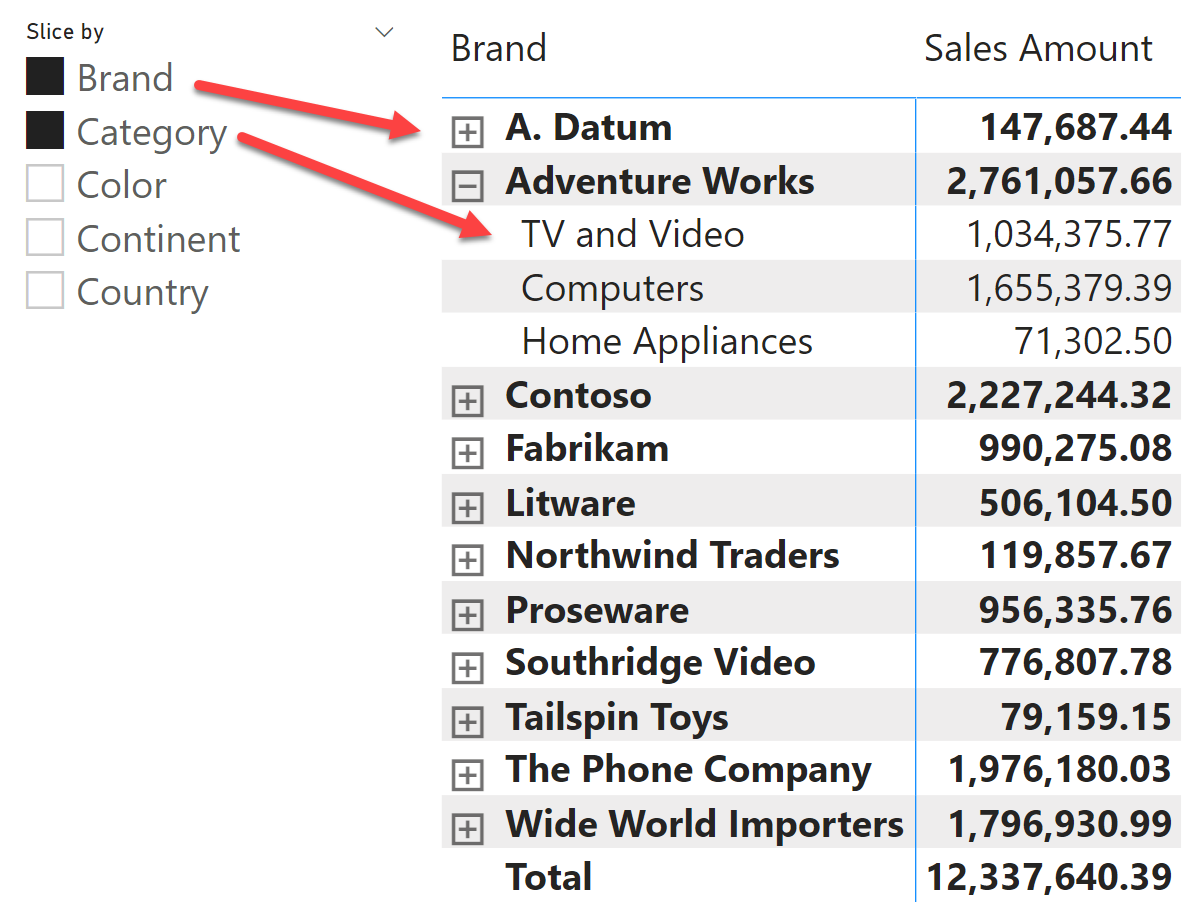
Fields parameters is a feature that allows users to choose which column to use to slice and dice values in a Power BI visual. By creating a fields parameter you can very easily build a report where the user can slice by Brand and Category, as in the following figure.
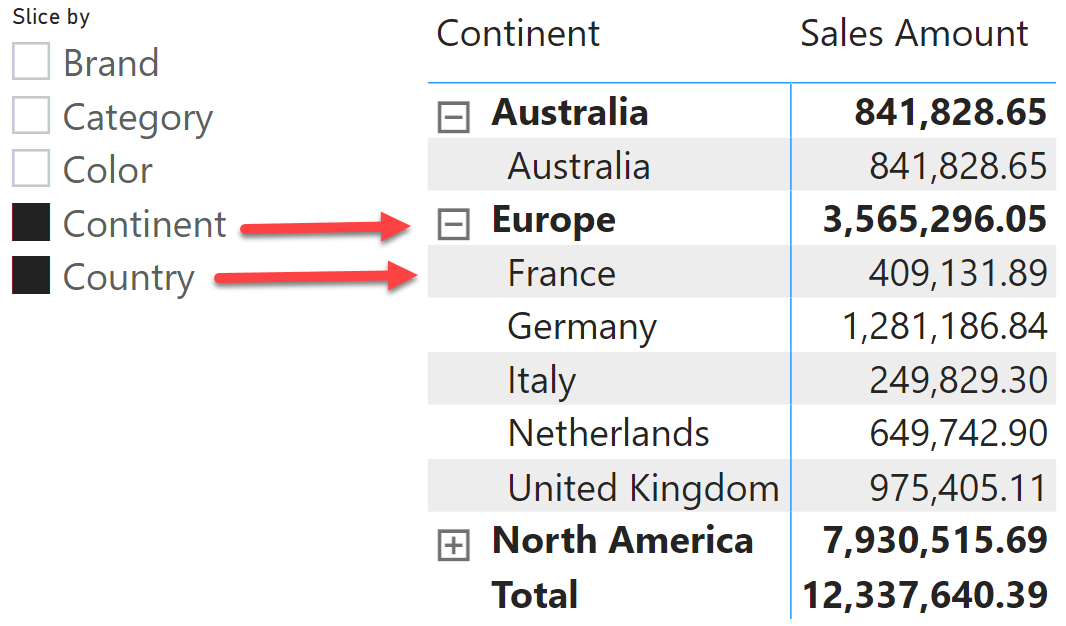
Or, by simply choosing a different selection in the slicer, the report slices by Continent and Country.
The feature itself is extremely simple to use. You create a new fields parameter and choose the columns that need to be part of the user selection.
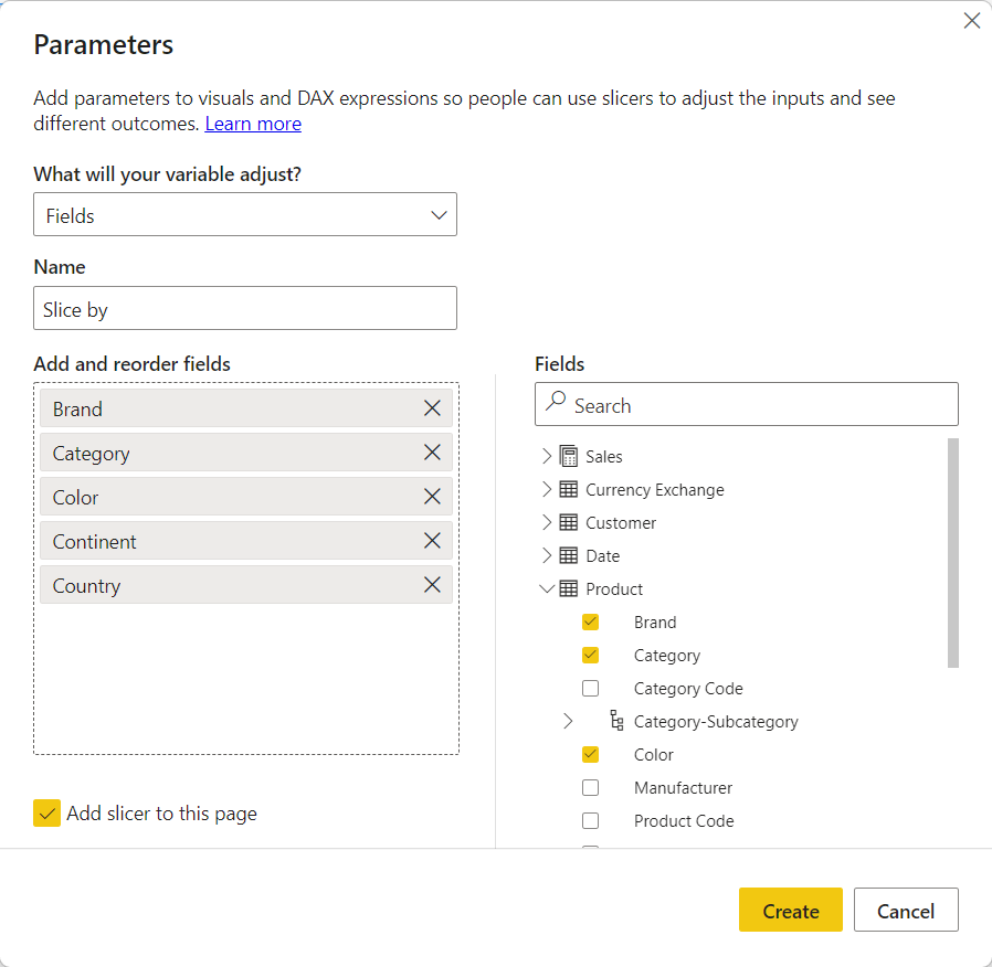
You also have the option of choosing the order of the fields, to optimize the user experience. This creates a new table in the model, with the name you provided (Slice by in the example above) which can be used to obtain dynamic slicing.
In order to achieve dynamic slicing, you need to use the Slice by column in the newly created table in a visual – a matrix, in our example – and use a slicer to choose the desired columns.
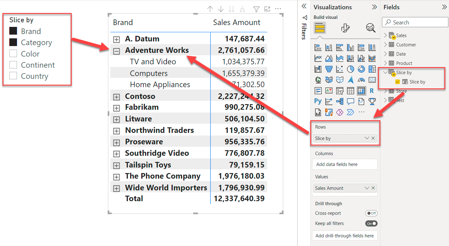
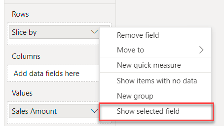
When you add a fields parameter to a visual, its aggregation is set by default to Show selected field. This indicates the special behavior introduced by Power BI to replace the fields parameter with the set of columns selected through the slicer.
The feature itself is very simple to use and very powerful at the same time. In this article, we are mainly interested in discovering the technical details of its implementation, so to have a better understanding of how it works.
Upon creating the parameter, Power BI creates a new calculated table using the following code:
1 2 3 4 5 6 7 8 | Slice by ={ ("Brand", NAMEOF('Product'[Brand]), 0), ("Category", NAMEOF('Product'[Category]), 1), ("Color", NAMEOF('Product'[Color]), 2), ("Continent", NAMEOF('Customer'[Continent]), 3), ("Country", NAMEOF('Customer'[Country]), 4)} |
 Copy
Copy Conventions
The table contains three columns: the name to display in the slicer, the name of the column that needs to be used, and the sort order. If you need to later change the parameter, you will need to edit this code manually. At the time of writing, there is no user interface to modify a fields parameter. Nonetheless, updating the content of the table is straightforward.
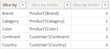
The only detail to note is the usage of the NAMEOF function. NAMEOF returns the fully qualified name of an object. Indeed, you can look at the content of the table using the data view, and find no surprises there.
The reason the generated code uses NAMEOF is that the table is automatically updated with new names in case you change the original column name. If at some point you rename the Product[Color] column to a different name, then the Power BI engine will propagate the rename operation to any DAX formula, including this calculated table. Therefore, using NAMEOF ensures the stability of your model even in case you perform updates later on.
The calculated table generated by Power BI contains additional metadata that informs Power BI of its role as a parameter table. We will go deeper on the topic later in this article. For now, we want to understand how Power BI uses a parameter table to execute the query.
By using Performance Analyzer, we can inspect the queries executed to produce the matrix. Quite surprisingly, the visual is rendered through the execution of two queries, instead of the usual single query per visual. This is the code as generated by Performance Analyzer:
1 2 3 4 5 6 7 8 9 10 11 12 13 14 15 16 17 18 19 20 21 22 23 24 25 26 27 28 29 30 31 32 33 34 35 36 37 | DEFINE VAR __DS0FilterTable = TREATAS ( { "'Customer'[Continent]", "'Customer'[Country]" }, 'Slice by'[Slice by Fields] ) VAR __DM3FilterTable = TREATAS ( { "Australia", "Europe", "North America" }, 'Customer'[Continent] ) VAR __DS0Core = SUMMARIZECOLUMNS ( ROLLUPADDISSUBTOTAL ( 'Customer'[Continent], "IsGrandTotalRowTotal", 'Customer'[Country], "IsDM1Total", NONVISUAL ( __DM3FilterTable ) ), __DS0FilterTable, "Sales_Amount", 'Sales'[Sales Amount] ) VAR __DS0PrimaryWindowed = TOPN ( 502, __DS0Core, [IsGrandTotalRowTotal], 0, 'Customer'[Continent], 1, [IsDM1Total], 0, 'Customer'[Country], 1 )EVALUATE__DS0PrimaryWindowedORDER BY [IsGrandTotalRowTotal] DESC, 'Customer'[Continent], [IsDM1Total] DESC, 'Customer'[Country] |
1 2 3 4 5 6 7 8 9 10 11 12 13 14 15 16 17 18 19 20 21 22 23 24 25 26 27 28 29 30 31 | DEFINE VAR __DS0FilterTable = TREATAS ( { "'Customer'[Continent]", "'Customer'[Country]" }, 'Slice by'[Slice by Fields] ) VAR __DS0Core = CALCULATETABLE ( SUMMARIZE ( 'Slice by', 'Slice by'[Slice by Fields], 'Slice by'[Slice by Order], 'Slice by'[Slice by] ), KEEPFILTERS ( __DS0FilterTable ) ) VAR __DS0BodyLimited = TOPN ( 152, __DS0Core, 'Slice by'[Slice by Order], 1, 'Slice by'[Slice by Fields], 1, 'Slice by'[Slice by], 1 )EVALUATE__DS0BodyLimitedORDER BY 'Slice by'[Slice by Order], 'Slice by'[Slice by Fields], 'Slice by'[Slice by] |
Because Performance Analyzer shows the queries in an order opposite to the order in which they are executed, and the code is somewhat complex to read, we also show a cleaned up version of the code. Here is the cleaned up version, with the execution order restored, which we will use for our analysis:
1 2 3 4 5 6 7 8 9 10 11 12 13 14 15 16 17 18 19 20 | ---- DAX Query to retrieve the column names--DEFINE VAR __DS0FilterTable = TREATAS ( { "'Customer'[Continent]", "'Customer'[Country]" }, 'Slice by'[Slice by Fields] )EVALUATECALCULATETABLE ( SUMMARIZE ( 'Slice by', 'Slice by'[Slice by Fields], 'Slice by'[Slice by Order], 'Slice by'[Slice by] ), KEEPFILTERS ( __DS0FilterTable )) |
1 2 3 4 5 6 7 8 9 10 11 12 13 14 | ---- DAX Query to produce the visual--EVALUATESUMMARIZECOLUMNS ( ROLLUPADDISSUBTOTAL ( 'Customer'[Continent], "IsGrandTotalRowTotal", 'Customer'[Country], "IsDM1Total" ), TREATAS ( { "Australia", "Europe", "North America" }, 'Customer'[Continent] ), "Sales_Amount", 'Sales'[Sales Amount]) |
As you see, there are two queries. The first one is querying the parameter table, retrieving the three columns, filtered by the slicer. Its output is the following.
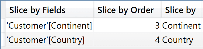
The result of this query is then used by Power BI to build the query that actually populates the visual, which no longer references the parameters – it slices directly by Continent and Country, producing the output for the visual.
This behavior is important to acknowledge. Indeed, using a parameter instead of a regular selection of columns in a visual does not have a performance impact on the query – except for the tiny amount of time required to gather the column names to be used in the query. Once Power BI retrieves the names, the query executed is identical to a query executed for a matrix without fields parameters.
At the same time, the two-step algorithm also means that the feature is expected to work based on client-tool interaction. A fields parameter is not part of the model, it is a piece of information that the client tool needs to use in order to execute the proper query. If the client tool does not support querying through a fields parameter, then the feature will not work. The first noticeable exception is Excel. Excel uses MDX to populate pivot tables, and it does not acknowledge fields parameters. Therefore, the fields parameter feature cannot be used in an Excel pivot table. Excel may or may not be updated in the future to take advantage of that feature. The important detail here is that if the client tool does not use the information, then the feature simply does not work. Currently, Power BI is the only tool making use of the metadata about fields parameters.
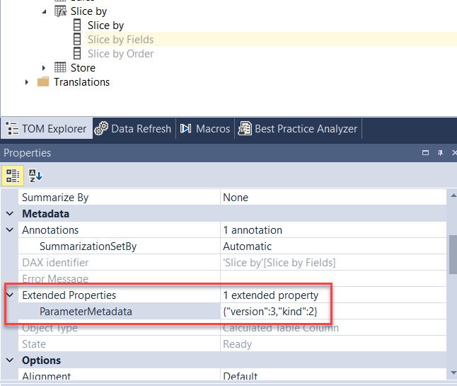
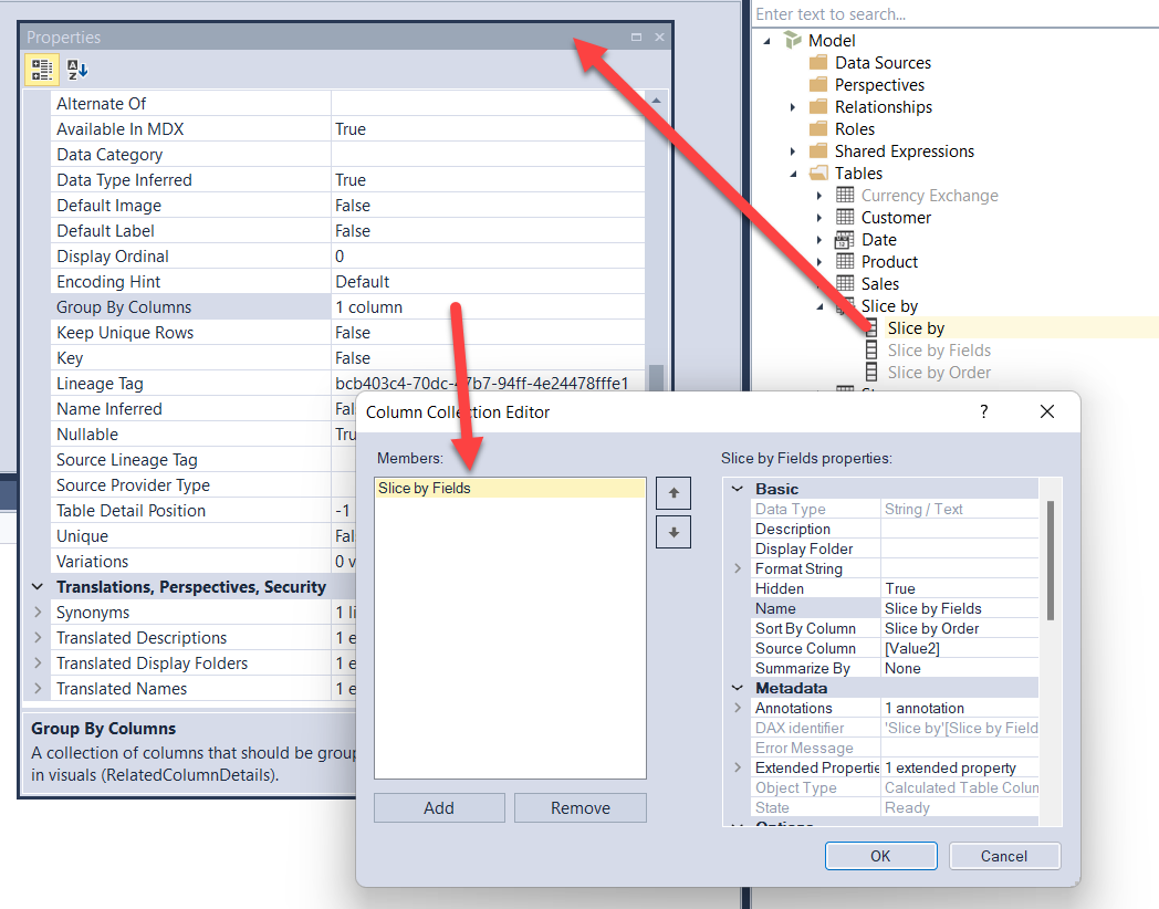
Let us now take a deeper look at the metadata required to let Power BI recognize a table as a parameter table. If we use Tabular Editor to inspect the content of the model, we notice a few details. What makes the table a parameter table are two important details: In the hidden Slice by Fields column there needs to be an extended property named ParameterMetadata, and the Slice By column (the column used in the slicer) needs to be grouped by the Fields column.
Here is the extended property of the Slice by Fields column where you see the first important detail.
And here the second important detail: the Slice by column needs to be grouped by Slice by Fields.
If you build a table and set its properties the right way, Power BI recognizes the table as a parameter table and behaves accordingly. Beware that this behavior is currently not documented, therefore it is subject to change in the future without notice. Nonetheless, if you need to create a parameter table programmatically without using the user interface, this technique works – at the time of writing, mind you.
Conclusions
Fields parameters are extremely useful, as they let users seamlessly change the columns used in a visual. Combined with calculation groups to change the measure being displayed, fields parameters may provide a very customizable user experience with minimal development effort. Their only shortcoming is that they currently work only in Power BI. Excel still needs regular pivot table editing to achieve an equivalent goal.
Returns the name of a column or measure.
NAMEOF ( <Value> )