 Marco Russo & Alberto Ferrari
What products did not sell in a specific area, store, or time period? This may be an important analysis for several businesses. There are multiple ways to obtain the desired result. Some specific implementations might be needed because of the user or model requirements, whereas developers can choose any formula in several cases. Or you might just find a solution on the web and blindly implement it without questioning whether there is a better way to achieve what you want.
It turns out that different formulas perform very differently. Choosing the right one in your scenario can make a slow report fast. This article analyzes the performance of different formulations of one same algorithm. Some are simple, some are rather complex. The takeaway of the article is not which formula runs best, but rather how to measure the performance of your measures and how relevant it is to execute performance analysis before putting a measure in production.
We want a measure that checks whether a product has no sales. The first implementation that comes to mind is to just use the Sales Amount measure and compare its value to zero:
DEFINE
    MEASURE Sales[HasNoSales] =
        [Sales Amount] = 0
EVALUATE
FILTER (
    SUMMARIZECOLUMNS (
        'Date'[Year],
        'Date'[Month Number],
        'Product'[Product Name],
        "Has no sales", [HasNoSales 0]
    ),
    [Has no sales] = TRUE ()
)
ORDER BY
    'Date'[Year],
    'Date'[Month Number]
The resulting report shows the products that – in a specific month – have no sales.
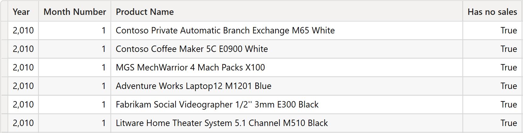
We are using Contoso 100M, which is a version of Contoso with around 200 million rows in Sales. When you test the queries with the downloadable demo file (which contains just a few thousand rows in Sales) your results may differ, but we needed a large database to execute the performance tests.
Before accepting this first attempt as the final solution, we want to test other formulas to obtain the same result. We have a total of six possible solutions. You might be more creative and find more, we stopped at six. The following is the full query containing the six measures. We execute the same query by just changing the line in SUMMARIZECOLUMNS that references the measure to test:
DEFINE
    MEASURE Sales[HasNoSales Sales Amount] = [Sales Amount] = 0
    MEASURE Sales[HasNoSales COUNTROWS] =
        COUNTROWS ( Sales ) = 0
    MEASURE Sales[HasNoSales ISEMPTY] =
        ISEMPTY ( Sales )
    MEASURE Sales[HasNoSales INTERSECT] =
        ISEMPTY (
            INTERSECT ( VALUES ( 'Product'[ProductKey] ), VALUES ( Sales[ProductKey] ) )
        )
    MEASURE Sales[HasNoSales EXCEPT] =
        NOT ISEMPTY (
            EXCEPT ( VALUES ( 'Product'[ProductKey] ), VALUES ( Sales[ProductKey] ) )
        )
    MEASURE Sales[HasNoSales SELECTEDVALUE] =
        NOT ( SELECTEDVALUE ( 'Product'[ProductKey] ) IN VALUES ( Sales[ProductKey] ) )

EVALUATE
FILTER (
    SUMMARIZECOLUMNS (
        'Date'[Year],
        'Date'[Month Number],
        'Product'[Product Name],
        "Has no sales", [HasNoSales Sales Amount]
    ),
    [Has no sales] = TRUE ()
)
ORDER BY
    'Date'[Year],
    'Date'[Month Number]
A few notes about the different measures – they all start with HasNoSales, followed by a suffix:
- Sales Amount: Our first test checks whether the value of Sales Amount is equal to zero.
- COUNTROWS: Instead of computing Sales Amount, it counts the number of rows in Sales to check that there are no rows in the filter context.
- ISEMPTY: Same as COUNTROWS, but it uses the ISEMPTY function to check that there are no rows.
- INTERSECT: It performs the intersection of the product keys in Sales and in Product, checking that there are no matching rows.
- EXCEPT: Similar to INTERSECT, but it uses EXCEPT to check that there are rows in Product that are not referenced in Sales.
- SELECTEDVALUE: It uses SELECTEDVALUE and the IN operator to check that the currently-selected product is not present among the products sold.
As you see, a simple measure like HasNoSales offers multiple possible implementations. Choosing the right one requires extensive testing. We look at the algorithm for each measure and perform some considerations.
Testing HasNoSales Sales Amount
The first measure just checks that Sales Amount is zero:
DEFINE
    MEASURE Sales[HasNoSales Sales Amount] = [Sales Amount] = 0
EVALUATE
FILTER (
    SUMMARIZECOLUMNS (
        'Date'[Year],
        'Date'[Month Number],
        'Product'[Product Name],
        "Has no sales", [HasNoSales Sales Amount]
    ),
    [Has no sales] = TRUE ()
)
ORDER BY
    'Date'[Year],
    'Date'[Month Number]
The server timings pane shows three different VertiPaq queries.
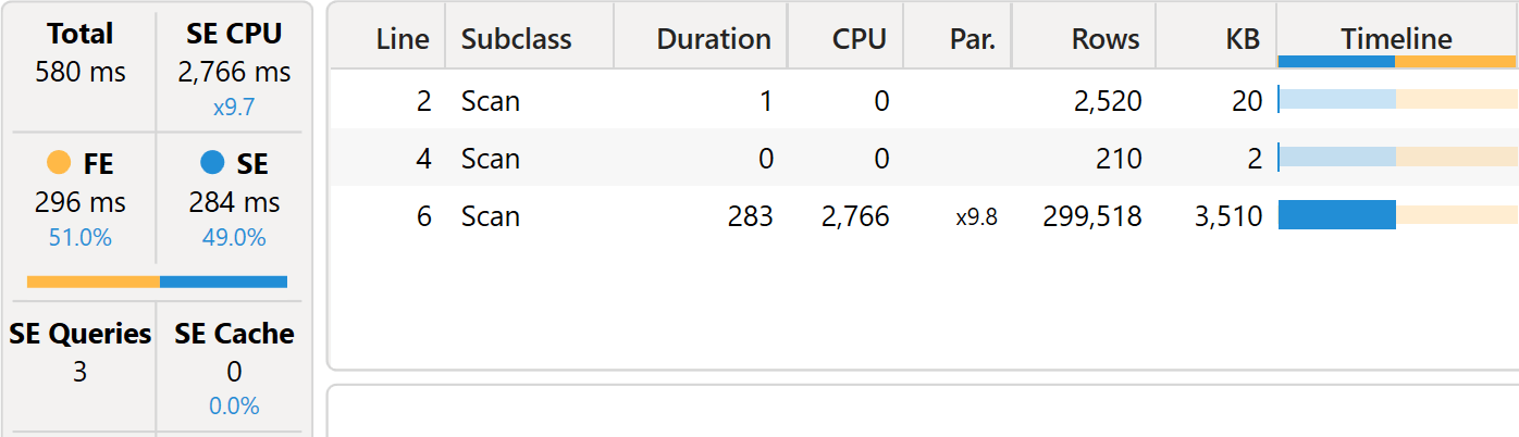
The first two queries are trivial, they retrieve the product names and the combinations of year and month number. They are so fast that it is not interesting to analyze them. The third xmSQL query is where the real work is:
WITH
    $Expr0 := ( PFCAST ( 'Sales'[Quantity] AS INT ) * PFCAST ( 'Sales'[Net Price] AS INT ) )
SELECT
    'Date'[Year],
    'Date'[Month Number],
    'Product'[Product Name],
    SUM ( @$Expr0 )
FROM 'Sales'
    LEFT OUTER JOIN 'Date'
        ON 'Sales'[Order Date]='Date'[Date]
    LEFT OUTER JOIN 'Product'
        ON 'Sales'[ProductKey]='Product'[ProductKey];
This query implements the full SUMMARIZECOLUMNS, as it computes the sales amount for all combinations of Year, Month, and Product Name. Once the storage engine computes the result, the formula engine removes zeroes and returns the result.
Because we are evaluating performance, the two important numbers are SE CPU (2,766 milliseconds) and FE (296 milliseconds). The total execution time is strongly affected by parallelism, so we do not look at the total execution time alone, as it would be a weak efficiency indicator.
Testing HasNoSales COUNTROWS
The second measure uses a different algorithm. Assuming that it is enough to check for the presence of rows in Sales to detect whether a product has sales, it expresses the algorithm by counting the number of rows in Sales and verifying that there are zero rows:
DEFINE
    MEASURE Sales[HasNoSales COUNTROWS] =
        COUNTROWS ( Sales ) = 0
EVALUATE
FILTER (
    SUMMARIZECOLUMNS (
        'Date'[Year],
        'Date'[Month Number],
        'Product'[Product Name],
        "Has no sales", [HasNoSales COUNTROWS]
    ),
    [Has no sales] = TRUE ()
)
ORDER BY
    'Date'[Year],
    'Date'[Month Number]
The assumption works as long as the Sales table contains only sales transactions. For example, if Sales also contained returns (with negative values), this second version would not be a good option. However, if the assumption is valid, we expect this second measure to be faster, as it does not multiply Quantity by Net Price.
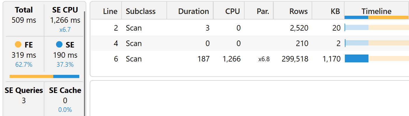
Indeed, this second measure runs faster.

The difference is all in the storage engine CPU: it went from 2,766 milliseconds down to 1,203 milliseconds, less than half the time. The first two queries are the same as the previous ones; the third xmSQL query shows that – this time – Sales Amount is not being computed:
SELECT
    'Date'[Year],
    'Date'[Month Number],
    'Product'[Product Name],
    COUNT ( )
FROM 'Sales'
    LEFT OUTER JOIN 'Date'
        ON 'Sales'[Order Date]='Date'[Date]
    LEFT OUTER JOIN 'Product'
        ON 'Sales'[ProductKey]='Product'[ProductKey];
There is still room for improvement. Testing COUNTROWS for zero requires the DAX engine to compute the number of sales transactions for each combination of year, month, and product included in the report. The only goal of this measure is to compare that number with zero to return True or False. The ISEMPTY function in DAX is optimized to check for the presence of rows in a table. ISEMPTY does not compute the number of rows; the presence of just one row implies that ISEMPTY returns FALSE. We use this approach in the following version of the measure.
Testing HasNoSales ISEMPTY
The third measure uses the same algorithm as the second, this time using ISEMPTY to check the presence of rows in Sales:
DEFINE
    MEASURE Sales[HasNoSales ISEMPTY] =
        ISEMPTY ( Sales )
EVALUATE
FILTER (
    SUMMARIZECOLUMNS (
        'Date'[Year],
        'Date'[Month Number],
        'Product'[Product Name],
        "Has no sales", [HasNoSales ISEMPTY]
    ),
    [Has no sales] = TRUE ()
)
ORDER BY
    'Date'[Year],
    'Date'[Month Number]
The measure makes the same assumptions as before. We hope that ISEMPTY produces a better execution plan. Unfortunately, that is not the case.
The difference in terms of speed is irrelevant. There is a small difference in the xmSQL queries, but it is insufficient to improve the overall speed. This third xmSQL query shows that the engine is not counting the number of rows because it is enough to check whether there are any rows:
SELECT
    'Date'[Year],
    'Date'[Month Number],
    'Product'[Product Name]
FROM 'Sales'
    LEFT OUTER JOIN 'Date'
        ON 'Sales'[Order Date]='Date'[Date]
    LEFT OUTER JOIN 'Product'
        ON 'Sales'[ProductKey]='Product'[ProductKey];
The COUNT of rows disappeared from xmSQL. Due to how data is compressed in VertiPaq, counting the rows in a table is very fast. It is so fast that there are no noticeable differences between whether the count is performed or not. However, with a different data distribution or a different type of compression, the time to count the number of rows might become relevant. Hence, we prefer this third version over the previous ones because its implementation produces a slightly simpler query plan.
The last three versions of the measure use a different algorithm. The idea is to leverage set functions in DAX to check whether they perform better or worse than the basic functions we have used. As we are about to find out, they are almost always worse. However, we always need to test the performance of different implementations before making any decision.
Testing HasNoSales INTERSECT
The fourth measure uses a different algorithm. We already know that ISEMPTY is a good function, so we use it to test whether the currently selected set of products intersected with the set of sold products produces an empty set. If the product has sales, it is included in VALUES ( Product[ProductKey] ) and will be part of the result when intersected with VALUES ( Sales[ProductKey] ). ISEMPTY checks whether the result of INTERSECT contains any row:
DEFINE
    MEASURE Sales[HasNoSales INTERSECT] =
        ISEMPTY (
            INTERSECT ( VALUES ( 'Product'[ProductKey] ), VALUES ( Sales[ProductKey] ) )
        )
EVALUATE
FILTER (
    SUMMARIZECOLUMNS (
        'Date'[Year],
        'Date'[Month Number],
        'Product'[Product Name],
        "Has no sales", [HasNoSales INTERSECT]
    ),
    [Has no sales] = TRUE ()
)
ORDER BY
    'Date'[Year],
    'Date'[Month Number]
We know that the formula engine computes set functions in DAX. However, it might be the case that the query plan shows improvements. Unfortunately, that is not the case.
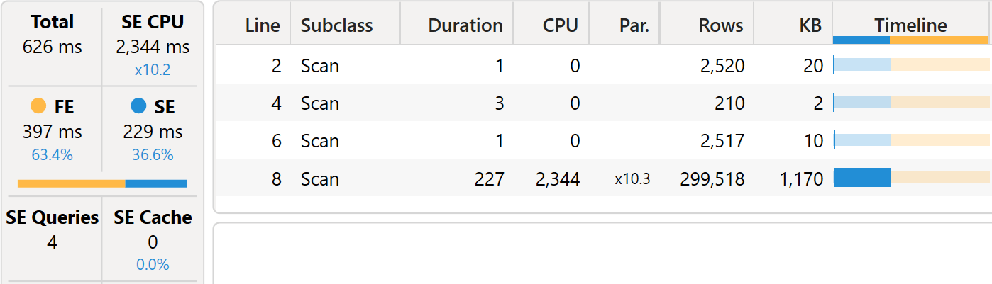
The storage engine CPU time has increased significantly and there are now four xmSQL queries instead of the earlier three. The first two xmSQL queries still retrieve products and months. The third one is interesting:
SELECT
    'Product'[ProductKey],
    'Product'[Product Name]
FROM 'Product';
This query retrieves the association between product keys and product names. Indeed, the DAX query groups by Product[Product Name], but the measure retrieves the set of product keys correctly. Therefore, the engine maps product names to product keys, adding complexity to the query plan.
The last query is very similar to the third version, with the increased complexity that it retrieves the combinations of year, month, product name, and product key – whereas the one used in HasNoSales ISEMPTY did not need the product key:
SELECT
    'Date'[Year],
    'Date'[Month Number],
    'Product'[Product Name],
    'Sales'[ProductKey]
FROM 'Sales'
    LEFT OUTER JOIN 'Date'
        ON 'Sales'[Order Date]='Date'[Date]
    LEFT OUTER JOIN 'Product'
        ON 'Sales'[ProductKey]='Product'[ProductKey];
This small difference is enough to increase the execution time of the entire query. The formula engine query plan is very close to the previous version.
From the analysis, it becomes clear that the problem with set functions is that we had to include references to Product[ProductKey] in the code. With the previous three formulas, the DAX code of the measures did not depend on a specific column. Therefore, the optimizer builds storage engine queries using only the columns present in the SUMMARIZECOLUMNS function. The set functions add complexity by forcing the engine to retrieve the product keys. It is very unlikely that the SUMMARIZECOLUMNS in the query uses ProductKey (users should use that column in the visual). Therefore, no matter what, the measures based on set functions are expected to be slower.
Testing HasNoSales EXCEPT
The fifth measure is a slight variation of the previous one. The difference is only in using EXCEPT rather than INTERSECT, which requires us to negate ISEMPTY:
DEFINE
    MEASURE Sales[HasNoSales EXCEPT] =
        NOT ISEMPTY (
            EXCEPT ( VALUES ( 'Product'[ProductKey] ), VALUES ( Sales[ProductKey] ) )
        )
EVALUATE
FILTER (
    SUMMARIZECOLUMNS (
        'Date'[Year],
        'Date'[Month Number],
        'Product'[Product Name],
        "Has no sales", [HasNoSales EXCEPT]
    ),
    [Has no sales] = TRUE ()
)
ORDER BY
    'Date'[Year],
    'Date'[Month Number]
Apart from the function used to process the results of the two VALUES functions, this formula is nearly identical to the previous one. Consequently, we expect to witness a similar level of performance.
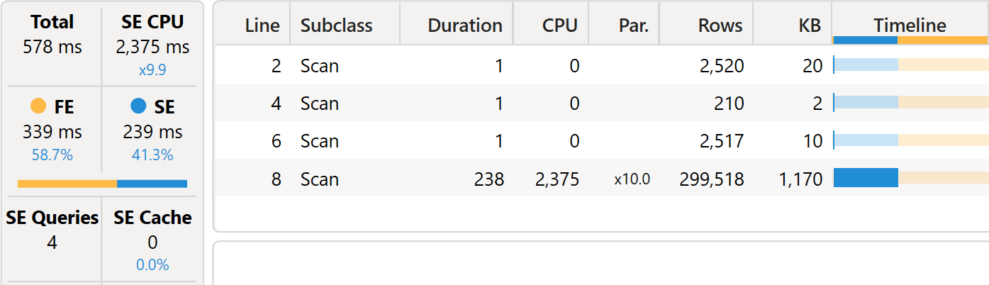
The xmSQL queries and the formula engine query plan are nearly identical to the previous version using INTERSECT. Consequently, server timings are basically the same.
Testing HasNoSales SELECTEDVALUE
The last measure to analyze uses the IN operator rather than a set function. It assumes that the external query computes the result for one product only – that is, the external SUMMARIZECOLUMNS is grouping at the Product level:
DEFINE
    MEASURE Sales[HasNoSales SELECTEDVALUE] =
        NOT ( SELECTEDVALUE ( 'Product'[ProductKey] ) IN VALUES ( Sales[ProductKey] ) )
EVALUATE
FILTER (
    SUMMARIZECOLUMNS (
        'Date'[Year],
        'Date'[Month Number],
        'Product'[Product Name],
        "Has no sales", [HasNoSales SELECTEDVALUE]
    ),
    [Has no sales] = TRUE ()
)
ORDER BY
    'Date'[Year],
    'Date'[Month Number]
Despite it looking quite close to previous versions, its performance is terrible.
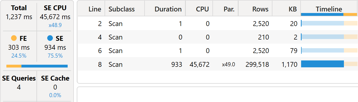
The storage engine CPU skyrocketed to 45,672 milliseconds. The reason is that the main xmSQL query now includes a callback:
SELECT
    'Date'[Year],
    'Date'[Month Number],
    'Product'[Product Name]
FROM 'Sales'
    LEFT OUTER JOIN 'Date'
        ON 'Sales'[Order Date]='Date'[Date]
    LEFT OUTER JOIN 'Product'
        ON 'Sales'[ProductKey]='Product'[ProductKey]
WHERE
    [CallbackDataID ( VALUES ( Sales[ProductKey] ) ) ] ( PFDATAID ( 'Product'[Product Name] ) , PFDATAID ( 'Sales'[ProductKey] ) ) ;
The measure is so slow that it is not worth investigating it further.
Conclusions
It is time to draw some conclusions. We summarized our findings in a table highlighting our favorite formula:
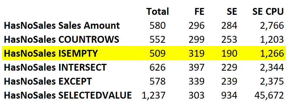
HasNoSales ISEMPTY seems a bit slower than HasNoSales COUNTROWS. However, be mindful that the difference is irrelevant, as it is way below the standard variation between different executions. The ISEMPTY version shows an xmSQL query slightly simpler than the COUNTROWS version, which explains our choice.
The important takeaway of the article is not that the ISEMPTY version is the best. The takeaway is that you must perform extensive testing before choosing one algorithm over another. The ratio between the best and the worst options in our portfolio of algorithms is around 40 – meaning that if we blindly choose the worst option, we potentially use 40 times the CPU power we would use had we chosen the best option.
Moreover, these are our findings on our demo database. We would not be surprised if you find different results on your own model because of size, data distribution, level of compression, and so on. When performance is critical, be prepared to perform extensive testing before going to production with a measure, no matter how simple that looks.
Create a summary table for the requested totals over set of groups.
SUMMARIZECOLUMNS ( [<GroupBy_ColumnName> [, [<FilterTable>] [, [<Name>] [, [<Expression>] [, <GroupBy_ColumnName> [, [<FilterTable>] [, [<Name>] [, [<Expression>] [, … ] ] ] ] ] ] ] ] ] )
Counts the number of rows in a table.
COUNTROWS ( [<Table>] )
Returns true if the specified table or table-expression is Empty.
ISEMPTY ( <Table> )
Returns the rows of left-side table which appear in right-side table.
INTERSECT ( <LeftTable>, <RightTable> )
Returns the rows of left-side table which do not appear in right-side table.
EXCEPT ( <LeftTable>, <RightTable> )
Returns the value when there’s only one value in the specified column, otherwise returns the alternate result.
SELECTEDVALUE ( <ColumnName> [, <AlternateResult>] )
Counts the number of rows in the table where the specified column has a non-blank value.
COUNT ( <ColumnName> )
When a column name is given, returns a single-column table of unique values. When a table name is given, returns a table with the same columns and all the rows of the table (including duplicates) with the additional blank row caused by an invalid relationship if present.
VALUES ( <TableNameOrColumnName> )