 Marco Russo & Alberto Ferrari
NOTE: this article is an excerpt of the Optimizing DAX book and video course.
Calculations that use the DAX time intelligence functions mostly retrieve data at the day level, performing the required aggregations in the formula engine. By avoiding time intelligence DAX functions, you can force DAX to produce more optimized queries for your specific calculations.
DirectQuery over SQL and VertiPaq require the same patterns to optimize time intelligence calculations, even though the reasons are different. In VertiPaq, we try to stay away from DAX time intelligence functions to avoid large materialization at the day level. With SQL, materialization does not always happen because Tabular tries to push the grouping down to SQL. Still, time intelligence calculations often result in complex queries, and it is better to avoid the complexity by using simpler DAX code.
As an example, let us analyze a DAX query that for each month computes the growth in sales compared with the same month in the previous year:
DEFINE
    MEASURE Sales[Sales PY] =
        CALCULATE ( [Sales Amount], SAMEPERIODLASTYEAR ( 'Date'[Date] ) )
EVALUATE
SUMMARIZECOLUMNS (
    'Date'[Year Month],
    'Date'[Year Month Number],
    "Sales Growth %", DIVIDE ( [Sales Amount] - [Sales PY], [Sales PY] )
)
ORDER BY 'Date'[Year Month Number]
The query runs in around 3.2 seconds.
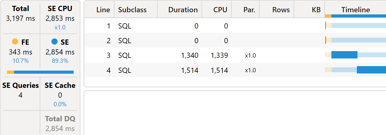
Most of the work happens inside SQL Server, even though the formula engine carries on some of the activities and consuming 10% of the overall execution time.
The first two SQL queries are trivial, as they only gather the dates and the relationship between dates and months. The first query returns the list of dates:
SELECT TOP (1000001) [t1].[Date]
FROM ([dbo].[Date]) AS [t1]
GROUP BY [t1].[Date]
This second query retrieves the relationship between dates and months because SAMEPERIODLASTYEAR works at the date level. Therefore, the formula engine retrieves the dates present in the Date table for each month to shift them to the previous year:
SELECT TOP (1000001) [t1].[Date],
    [t1].[Year Month],
    [t1].[Year Month Number]
FROM ([dbo].[Date]) AS [t1]
GROUP BY [t1].[Date],
    [t1].[Year Month],
    [t1].[Year Month Number]
The third query retrieves sales at the date level. The original query is 3,679 lines long. We show just an excerpt:
SELECT TOP (1000001) *
FROM (
    SELECT [semijoin1].[c20],
        [semijoin1].[c22],
        SUM([a0]) AS [a0]
    FROM (
        (
            SELECT [t1_Date],
                [a0]
            FROM (
                SELECT [t1].[Date] AS [t1_Date],
                    [t3].[Quantity] AS [t3_Quantity],
                    [t3].[Net Price] AS [t3_Net Price],
                    ([t3].[Quantity] * [t3].[Net Price]) AS [a0]
                FROM (
                    [Data].[Sales] AS [t3]
                        LEFT JOIN [dbo].[Date] AS [t1] ON ([t3].[Order Date] = [t1].[Date])
                    )
                ) AS [t0]
            ) AS [basetable0]
            INNER JOIN (
            (SELECT N'January 2011' AS [c20], 24133 AS [c22],
                    CAST('20100101 00:00:00' AS DATETIME) AS [t1_Date])
            UNION ALL (SELECT N'January 2011' AS [c20], 24133 AS [c22],
                              CAST('20100102 00:00:00' AS DATETIME) AS [t1_Date])
            UNION ALL (SELECT N'January 2011' AS [c20], 24133 AS [c22],
                              CAST('20100103 00:00:00' AS DATETIME) AS [t1_Date])
...
            UNION ALL (SELECT N'December 2020' AS [c20], 24252 AS [c22],
                              CAST('20191230 00:00:00' AS DATETIME) AS [t1_Date])
            UNION ALL (SELECT N'December 2020' AS [c20], 24252 AS [c22],
                              CAST('20191231 00:00:00' AS DATETIME) AS [t1_Date])
            ) AS [semijoin1] ON (([semijoin1].[t1_Date] = [basetable0].[t1_Date]))
        )
    GROUP BY [semijoin1].[c20],
        [semijoin1].[c22]
    ) AS [MainTable]
WHERE (NOT (([a0] IS NULL)))
Despite being verbose, the query is relatively simple: it retrieves the sales amount grouped by month with a filter on the date that contains 9 years. Interestingly, the filter includes the group by columns for the current year, but the dates are in the previous year. If you focus on the first SELECT that filters the entire query, the values are January 2011 for the month name, 24133 for the month number, and January 1st, 2010 for the date. In other words, when the grouping happens for January 2011, the dates aggregated are in January 2010.
This detail is essential. It means that the grouping operation happens inside SQL. SQL must materialize an internal structure containing the sales amount by date, but it groups data at the month level and returns a small datacache containing only the result.
The last SQL query computes the sales amount at the month level:
SELECT TOP (1000001) *
FROM (
    SELECT [t1_Year Month],
        [t1_Year Month Number],
        SUM([a0]) AS [a0]
    FROM (
        SELECT [t1].[Year Month] AS [t1_Year Month],
            [t1].[Year Month Number] AS [t1_Year Month Number],
            [t3].[Quantity] AS [t3_Quantity],
            [t3].[Net Price] AS [t3_Net Price],
            ([t3].[Quantity] * [t3].[Net Price]) AS [a0]
        FROM (
            [Data].[Sales] AS [t3]
                LEFT JOIN [dbo].[Date] AS [t1] ON ([t3].[Order Date] = [t1].[Date])
            )
        ) AS [t0]
    GROUP BY [t1_Year Month],
        [t1_Year Month Number]
    ) AS [MainTable]
WHERE (NOT (([a0] IS NULL)))
As you see, the pattern in the communication between the storage engine and the formula engine is different from the one in VertiPaq. VertiPaq materializes data at the day level and groups by month in the formula engine, whereas DirectQuery groups data by month in the storage engine. However, the SQL query retrieving values from the previous year is quite complex.
We can perform in DirectQuery the same optimization applied to VertiPaq by using the Date[Year Month Number] mathematical properties to compute the sales in the previous year by just subtracting 12 from the current month:
DEFINE
    MEASURE Sales[Sales PY] =
        VAR CurrentMonth =
            MAX ( 'Date'[Year Month Number] )
        RETURN
            CALCULATE (
                [Sales Amount],
                REMOVEFILTERS ( 'Date' ),
                'Date'[Year Month Number] = CurrentMonth - 12
            )

EVALUATE
SUMMARIZECOLUMNS (
    'Date'[Year Month],
    'Date'[Year Month Number],
    "Sales Growth %", DIVIDE ( [Sales Amount] - [Sales PY], [Sales PY] )
)
ORDER BY 'Date'[Year Month Number]
This query lowers the execution time from 3.2 seconds to less than 2 seconds.
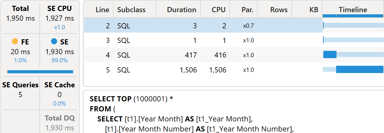
The first two SQL queries retrieve the basic columns from Date, and their execution time is irrelevant. This is the first one:
SELECT TOP (1000001) *
FROM (
    SELECT [t1].[Year Month] AS [t1_Year Month],
        [t1].[Year Month Number] AS [t1_Year Month Number],
        MAX([t1].[Year Month Number]) AS [a0]
    FROM ([dbo].[Date]) AS [t1]
    GROUP BY [t1].[Year Month],
        [t1].[Year Month Number]
    ) AS [MainTable]
WHERE (NOT (([a0] IS NULL)))
And this is the second SQL query:
SELECT TOP (1000001) [t1].[Year Month Number]
FROM ([dbo].[Date]) AS [t1]
GROUP BY [t1].[Year Month Number]
The third SQL query is much shorter than the equivalent for the previous DAX query:
SELECT TOP (1000001) *
FROM (
    SELECT [t1_Year Month Number],
        SUM([a0]) AS [a0]
    FROM (
        SELECT [t1].[Year Month Number] AS [t1_Year Month Number],
            [t3].[Quantity] AS [t3_Quantity],
            [t3].[Net Price] AS [t3_Net Price],
            ([t3].[Quantity] * [t3].[Net Price]) AS [a0]
        FROM (
            [Data].[Sales] AS [t3]
                LEFT JOIN [dbo].[Date] AS [t1] ON ([t3].[Order Date] = [t1].[Date])
            )
        ) AS [t0]
    WHERE (
            (
                [t1_Year Month Number] IN (
                    24128, 24168,
...
                    24173, 24215
                    )
                )
            )
    GROUP BY [t1_Year Month Number]
    ) AS [MainTable]
WHERE (NOT (([a0] IS NULL)))
The WHERE condition is more straightforward, as it involves a single column. Moreover, the grouping naturally happens inside SQL more simply than in the previous example. This results in a faster execution time that accounts for most of the time saved.
The last query retrieves the sales amount by year month, and it is very similar to the corresponding query for the previous DAX query:
SELECT TOP (1000001) *
FROM (
    SELECT [t1_Year Month],
        [t1_Year Month Number],
        SUM([a0]) AS [a0]
    FROM (
        SELECT [t1].[Year Month] AS [t1_Year Month],
            [t1].[Year Month Number] AS [t1_Year Month Number],
            [t3].[Quantity] AS [t3_Quantity],
            [t3].[Net Price] AS [t3_Net Price],
            ([t3].[Quantity] * [t3].[Net Price]) AS [a0]
        FROM (
            [Data].[Sales] AS [t3]
                LEFT JOIN [dbo].[Date] AS [t1] ON ([t3].[Order Date] = [t1].[Date])
            )
        ) AS [t0]
    GROUP BY [t1_Year Month],
        [t1_Year Month Number]
    ) AS [MainTable]
WHERE (NOT (([a0] IS NULL)))
Using regular, optimized DAX code rather than DAX time intelligence functions, we executed simpler SQL code that saved a considerable amount of time. The formula engine time also became irrelevant – 20 milliseconds against 343 when using SAMEPERIODLASTYEAR.
Before we move on from this topic, it is essential to note that the optimization of DAX time intelligence functions that reduces the size of the datacache to the month level does not always kick in. SAMEPERIODLASTYEAR and DATEADD benefit from this optimization: with these functions, the DirectQuery engine groups data at the time granularity required by the DAX query. Other DAX functions like DATESBETWEEN and DATESYTD, or more complex DAX queries, still require data to be returned to the formula engine at the day level.
As an example, look at the following DAX query. It implements the behavior of SAMEPERIODLASTYEAR through several variables and a DATESBETWEEN. Despite being functionally equivalent to the version with SAMEPERIODLASTYEAR, it requires data at the day level sent from the DirectQuery storage engine:
DEFINE
    MEASURE Sales[Sales PY] =
        VAR LastDay = MAX ( 'Date'[Date] )
        VAR EndSPLY = EOMONTH ( LastDay, -12 )
        VAR StartSPLY = EOMONTH ( LastDay, -13 ) + 1
        RETURN
            CALCULATE ( [Sales Amount], DATESBETWEEN ( 'Date'[Date], StartSPLY, EndSPLY ) )

EVALUATE
SUMMARIZECOLUMNS (
    'Date'[Year Month],
    'Date'[Year Month Number],
    "Sales Growth %", DIVIDE ( [Sales Amount] - [Sales PY], [Sales PY] )
)
ORDER BY 'Date'[Year Month Number]
It is not worth analyzing the entire query. The critical part is the code that retrieves information for the sales in the previous year, which is the following SQL query:
SELECT TOP (1000001) *
FROM (
    SELECT [t1_Date],
        SUM([a0]) AS [a0]
    FROM (
        SELECT [t1].[Date] AS [t1_Date],
            [t3].[Quantity] AS [t3_Quantity],
            [t3].[Net Price] AS [t3_Net Price],
            ([t3].[Quantity] * [t3].[Net Price]) AS [a0]
        FROM (
            [Data].[Sales] AS [t3]
                LEFT JOIN [dbo].[Date] AS [t1] ON ([t3].[Order Date] = [t1].[Date])
            )
        ) AS [t0]
    WHERE (
            (
                [t1_Date] IN (
                    CAST(‘20120812 00:00:00’ AS DATETIME),
                    CAST(‘20171219 00:00:00’ AS DATETIME),


                    CAST(‘20120922 00:00:00’ AS DATETIME),
                    CAST(‘20201203 00:00:00’ AS DATETIME)
                    )
                )
            )
    GROUP BY [t1_Date]
    ) AS [MainTable]
WHERE (NOT (([a0] IS NULL)))
The SQL query groups by Date; this increases the size of the datacache exchanged between SQL Server and the formula engine, consequently putting more pressure on the formula engine. As with any optimization pattern, the DAX engine can evolve, so testing on your specific version of Tabular is required before making any assumption.
To get the best performance in DirectQuery, DAX time intelligence functions should be avoided and, whenever possible, replaced with more basic code that can be controlled, seeking for the optimal query plan.
Returns a set of dates in the current selection from the previous year.
SAMEPERIODLASTYEAR ( <Dates> )
Moves the given set of dates by a specified interval.
DATEADD ( <Dates>, <NumberOfIntervals>, <Interval> )
Returns the dates between two given dates.
DATESBETWEEN ( <Dates>, <StartDate>, <EndDate> )
Returns a set of dates in the year up to the last date visible in the filter context.
DATESYTD ( <Dates> [, <YearEndDate>] )