 Kurt Buhler
In a previous article about format strings, we showed an example of how format strings can improve visualizations. The visualizations in that article compared the performance of a company’s marketing videos on a streaming platform to the average of all their videos released that year. In this article, we explain how to conduct this analysis yourself in DAX, where you compare series that occur in different periods.
This analysis compares the initial performance of two videos over time while accounting for the fact that the videos were published on different dates. Since videos on streaming platforms get the most views immediately after publication, we will focus this analysis on the first twenty weeks (five months).
Other scenarios where this might be relevant include:
- Comparing products or customers by sales for the weeks since the first sale, or the days since a marketing action.
- Comparing applications by incidents for the days since the release, or the days since reaching 1000 weekly active users.
- Comparing countries by cases of a virus for the days since reaching a certain number of confirmed cases.
Describing the Initial model
The input of the analysis is a Views fact table that shows the total views by week, and a Videos dimension table that contains descriptive attributes for each video. The two tables are related by the video ID.

If we want to compare the videos by the sum of all views, we can easily identify the top most-viewed videos:
Total Views =
SUM ( 'Views'[Views] )
We see the result when we view the Total Views by title, below.

This is not a very useful comparison, since older videos (as indicated by the red box) will have accumulated more views over time.
Viewing the data as a time series is not very valuable either, since views only start being recorded from the different publish dates of each video. The following example shows what this looks like when filtering to a six-month period.

This example shows the views over time for each video, but creating a line chart for this only produces a mess. The line chart on the left is cross-filtered to the top three videos, but even Sparklines (small multiple-line charts within a table) are no better because the y-axes are not aligned. So we can only compare very general trends, and not performance.
To achieve a valid comparison, we need to compare each video while controlling for the difference in periods.
Preparing the model
Ideally, we should find a way to standardize the timeline, so we can see the performance of each video since the date it was published. The first step is to create a column that describes the weeks since publication. This must be a column in the fact table, since the value differs for each transaction. We will then later use a dimension table to place Weeks Since Publication on the x-axis of a line chart:
Weeks Since Publication =
VAR _DateOfPublication =
    RELATED( 'Videos'[Publish Date] )

VAR _Weeks =
    ( 'Views'[Date] - _DateOfPublication ) / 7

RETURN
    _Weeks
This example shows how to create this column by using DAX, but you should preferentially do this upstream in Power Query, or in your data source by using SQL, PySpark, or whatever suits your needs, skills, and workflow best.
We should then create the dimension table, which we will relate to this Weeks Since Publication column. In the sample file, this is a simple calculated table:
Weeks =
VALUES ( Views[Weeks Since Publication] )
After the creation of the relationship, the model looks like the diagram below.

Next, we have to create the appropriate DAX measures to use in the analysis.
Creating the DAX measures
Next, since we are interested in total performance, we must create a measure to cumulate the weekly views by the Weeks Since Publication. In this measure, we include a condition to hide the value if the week is in the future:
Views Since Publication =
CALCULATE (
    [Total Views],
    FILTER (
        ALL ( 'Weeks'[Weeks Since Publication] ),
        'Weeks'[Weeks Since Publication] <= MAX ( 'Weeks'[Weeks Since Publication] )
    )
)
By plotting this measure in a line or area chart by Weeks Since Publication, we can see the views for a standardized timeline. Using a slicer, we can filter the chart to the first twenty weeks (since that is the period we are interested in). While this chart is useful to compare selected videos, we still have a problem: the number of videos is too high to compare all of them. The view is only useful if we filter to view only a few videos at a time.

To overcome this issue, we can instead plot the value for a single selected video (the one we are interested in analyzing) against the typical performance of all videos. Specifically, we will compare the views for a selected video against the average views of all videos released in the same year. The first step is to modify the Cumulative Weekly Views to only return a result when a single video is selected. This is not mandatory, but it ensures that users do not see an unexpected result when not selecting a video or forcing the selection of multiple videos:
Views Since Publication (Selected Title) =
VAR _LatestWeekWithViews = MAX ( 'Views'[Weeks Since Publication] )

VAR _SelectedWeek = SELECTEDVALUE ( 'Weeks'[Weeks Since Publication] )

RETURN
    IF (
        -- Only one video is selected
        HASONEVALUE ( 'Videos'[Title] )
            &&  -- The week in scope is not greater than the latest week with data
                NOT _SelectedWeek > _LatestWeekWithViews,
        [Views Since Publication]
    )
Next, we create a measure that computes the average cumulative views for all of the videos that have been published after a specific cutoff date:
Avg. Views Since Publication =
-- Filter out videos published before this date
VAR _DateCutoff = DATE ( 2022, 01, 01 )

VAR _SelectedWeek = SELECTEDVALUE ( 'Weeks'[Weeks Since Publication] )

VAR _LatestWeekWithViews =
    CALCULATE(
        MAX ( 'Views'[Weeks Since Publication] ),
        'Videos'[Publish Date] > _DateCutoff,
        ALL ( 'Videos' )
    )

VAR _Result =
    CALCULATE (
        AVERAGEX (
            VALUES ( 'Videos'[Title] ),
            [Views Since Publication]
        ),
        'Videos'[Publish Date] > _DateCutoff,
        ALL ( 'Videos' )
    )
RETURN
    IF (
        -- The week in scope is not greater than the latest week for which there is data
        NOT _SelectedWeek > _LatestWeekWithViews,
        _Result
    )
Formatting the visual
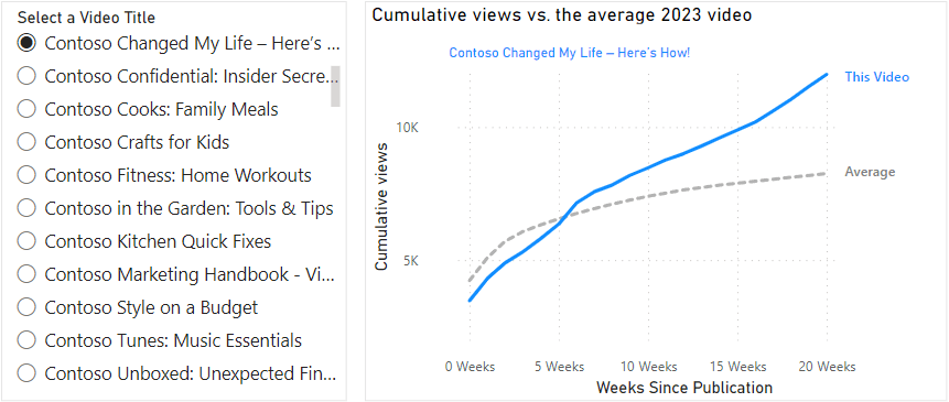
Once the model and measures are ready, we have the visualization below.

To set up the visuals, we should make adjustments to both the slicer and the line chart. In the slicer, we should enforce a single selection. Then, in the line chart, we add both Views Since Publication (Selected Video) and Avg. Views Since Publication to the “Values”. We can further improve the line chart by performing two formatting enhancements:
- Moving Title to “Small Multiples”, and formatting the small multiple title, accordingly. This ensures a dynamic title for the line chart dependent upon the slicer selection.
- Enabling “Series Labels”. This can be more clear compared to a traditional legend. To make the series label more useful, re-name in the “Values” area the Views Since Publication (Selected Video) measure to “This video” and re-name Views Since Publication to “Average”.
Following these steps produces our final result, which allows a dynamic comparison of videos to the average.
Conclusion
When you compare series that cover different periods, it is useful to standardize the timeline to a common event, such as a publication date. This ensures the series comparisons are valid and helps reveal trends, patterns, or outliers.